Advanced Strategies for EEG Artifact Reduction: A Comprehensive Guide for Biomedical Research and Drug Development
Clean electroencephalography (EEG) data is paramount for accurate analysis in neuroscience research and drug development.
Advanced Strategies for EEG Artifact Reduction: A Comprehensive Guide for Biomedical Research and Drug Development
Abstract
Clean electroencephalography (EEG) data is paramount for accurate analysis in neuroscience research and drug development. This article provides a comprehensive guide to reducing neural data artifacts in EEG recordings, tailored for researchers and drug development professionals. It begins by establishing a foundational understanding of diverse artifact types, from physiological sources like ocular and muscle activity to non-physiological technical noise. The core of the article explores a wide spectrum of artifact removal methodologies, from established signal processing techniques like Independent Component Analysis (ICA) to cutting-edge machine learning and deep learning models, including hybrid CNN-LSTM architectures. It further offers practical troubleshooting and optimization strategies for challenging recording environments, such as simultaneous EEG-fMRI, and provides a rigorous framework for the validation and comparative analysis of different denoising techniques. By synthesizing modern practices, this guide aims to enhance data integrity and reliability in pharmacokinetic/pharmacodynamic modeling and clinical neuroscience applications.
Understanding the Enemy: A Complete Guide to EEG Artifact Types and Origins
Frequently Asked Questions (FAQs)
Q1: What are the most common types of EEG artifacts I might encounter in my research? EEG artifacts are unwanted signals that originate from sources other than the brain's neuronal activity. They are broadly categorized as follows [1] [2]:
- Physiological Artifacts: Generated from the subject's own body.
- Ocular Artifacts: Caused by eye movements and blinks. They have high amplitude and are most prominent in frontal electrodes [1].
- Muscle Artifacts (EMG): Caused by tension in head, neck, or jaw muscles, such as talking or swallowing. They have a broad frequency range and can be very challenging to remove [1].
- Cardiac Artifacts (ECG): Caused by the electrical activity of the heart, often appearing as a periodic QRS-like pattern in the EEG [2].
- External/Environmental Artifacts: Arise from outside the subject.
Q2: My wearable EEG data is very noisy. Do standard artifact removal methods work for low-channel count, mobile setups? Wearable EEG presents specific challenges, including motion artifacts and signal degradation from dry electrodes. While standard methods are used, they require adaptation [3].
- Independent Component Analysis (ICA) is widely applied but its effectiveness can be limited by the reduced spatial resolution of low-density EEG arrays [3].
- Blind Source Separation (BSS) methods, including ICA, assume a sufficient number of channels to separate sources effectively, which is a limitation for low-channel count setups [4].
- Emerging deep learning approaches are showing promise for handling motion and muscular artifacts in real-time, wearable settings as they can learn features directly from the data without requiring a high channel count [3] [4].
- Auxiliary sensors, such as Inertial Measurement Units (IMUs), have great potential for detecting motion artifacts but are currently underutilized in practice [3].
Q3: How can I quickly check my raw EEG data for major artifacts before full processing? Visual inspection is a fundamental first step. You can use plotting functions in toolboxes like MNE-Python to browse your data [2]:
- Plot Raw Data: Scroll through the continuous data in a "vertical" viewmode to see all channels stacked. Look for large, abrupt deflections (eye blinks), high-frequency "bursts" (muscle noise), or regular, sharp patterns (cardiac artifacts) [2] [5].
- Check the Power Spectrum: Plot the power spectral density of your data. Look for sharp peaks at 50/60 Hz (power line noise) and its harmonics [2].
- Use a Databrowser: Tools like
ft_databrowserin FieldTrip or the MNE browsing interface allow you to visually mark and annotartifactual periods for later rejection [5].
Q4: When should I reject data segments versus using a correction algorithm? The choice depends on your research question and the extent of contamination [2] [6].
- Reject Epochs: This is the safest method when artifacts are large, infrequent, and short-lived. It is recommended when you have a sufficient number of clean trials remaining for analysis. Simply discarding contaminated epochs prevents the artifact from influencing your results.
- Repair with Algorithms: Use correction methods (e.g., ICA, regression, deep learning) when artifacts are frequent and rejecting them would lead to an unacceptable loss of data, or when the artifact overlaps with the neural signal of interest (e.g., a blink occurring during a key event-related potential) [6].
Troubleshooting Guides
Problem: Persistent Ocular (Eye Blink and Movement) Artifacts
Symptoms: Large, low-frequency deflections in frontal EEG channels, time-locked to eye blinks or movements.
Solutions:
- Independent Component Analysis (ICA): This is the most common and effective method [6].
- Procedure: Apply ICA to your multi-channel data to decompose it into independent components. Inspect the topography and time course of each component. Components showing a frontal pole topography and a waveform that matches blinks should be selected for removal. Reconstruct the signal without these artifactual components [6].
- Considerations: ICA works best with a sufficient number of channels and high-quality data. It requires manual component selection or a validated automated classifier.
- Regression in Time or Frequency Domain: This method requires a recorded EOG reference channel [1].
- Procedure: A transmission factor is calculated between the EOG reference and the EEG channels. The estimated artifact contribution is then subtracted from the EEG data [1].
- Considerations: A key limitation is that the EOG channel itself contains brain signals, so this method can subtract relevant neural activity along with the artifact [1].
Problem: Muscle Artifact (EMG) Contamination
Symptoms: High-frequency, irregular, and low-voltage activity that can be widespread or localized over temporal muscles.
Solutions:
- Automated Detection and Rejection: Use algorithms to identify and mark periods of high muscle activity.
- Procedure: Calculate metrics like amplitude, variance, or frequency features (e.g., power in the 20-60 Hz band) on sliding windows of data. Epochs where these metrics exceed a predefined threshold are marked for rejection [3].
Spatial Filtering and Source Separation: ICA can also separate and remove muscle artifacts [1] [6].
- Procedure: The decomposition process is similar to that for ocular artifacts. Muscle artifact components are often characterized by a high-frequency, "spiky" time course and a topography focused on the temporal areas. These components are removed before signal reconstruction [6].
Advanced Deep Learning Methods: Newer models are highly effective for this difficult artifact.
- Procedure: Use a pre-trained model like CLEnet, which integrates Convolutional Neural Networks (CNN) and Long Short-Term Memory (LSTM) networks to extract both morphological and temporal features of EEG, effectively separating clean neural signals from EMG contamination [4].
Problem: Power Line (50/60 Hz) and High-Frequency Noise
Symptoms: A persistent, oscillatory peak at 50 Hz or 60 Hz (and its harmonics at 120 Hz, 180 Hz, etc.) visible in the power spectrum.
Solutions:
- Notch Filtering: Apply a narrow band-stop filter centered precisely at the power line frequency (e.g., 50 Hz) [2].
- Caution: Notch filters can introduce ringing artifacts and may remove a small portion of neural signal in the same frequency band. Use them judiciously.
- SSP or SSPP: These projection-based methods are effective for removing periodic noise.
- Procedure: The method identifies the topographical pattern of the environmental noise and creates a projector that removes this pattern from the data [2].
Quantitative Data on Artifact Removal Techniques
Table 1: Performance Comparison of Modern Artifact Removal Algorithms (Based on Semi-Synthetic Data)
| Algorithm | Artifact Type | Key Metric: Signal-to-Noise Ratio (SNR) | Key Metric: Correlation Coefficient (CC) | Best For |
|---|---|---|---|---|
| CLEnet (CNN + LSTM) [4] | Mixed (EOG + EMG) | 11.50 dB | 0.925 | Multi-channel data with unknown artifacts |
| 1D-ResCNN [4] | Mixed (EOG + EMG) | Not Reported | ~0.90 (inferred) | Single-channel scale feature extraction |
| NovelCNN [4] | EMG | High Performance | High Performance | EMG-specific artifact removal |
| EEGDNet (Transformer) [4] | EOG | High Performance | High Performance | EOG-specific artifact removal |
| ICA (Traditional) [3] [6] | Ocular, Muscular | Varies with data | Varies with data | Multi-channel data with clear source topographies |
Table 2: Essential Research Reagent Solutions for EEG Experiments
| Item | Function / Purpose | Example Use-Case |
|---|---|---|
| 64-channel EEG cap (10-20 system) | High-density spatial sampling for source localization and effective ICA [7] | Auditory MMN studies in clinical populations [7] |
| Electrooculogram (EOG) electrodes | Provide reference signals for vertical and horizontal eye movements [1] [7] | Critical for regression-based ocular artifact correction or EOG-assisted ICA component identification [1] |
| Conductive Gel & Abrasive Prep Kits | Ensure low electrode-skin impedance (< 10 kΩ), reducing baseline noise and electrode artifacts [7] | Mandatory for all high-fidelity ERP studies, especially in clinical drug development [7] |
| Auditory Stimulation System | Precisely deliver standard and deviant tones for evoked potentials (e.g., MMN, P300) [7] | Investigating sensory processing deficits in schizophrenia or Alzheimer's disease [7] |
| Automated Artifact Detection Software (e.g., MNE, FieldTrip) | Perform filtering, epoching, and automated artifact rejection based on statistical thresholds [2] [5] | Standardizing preprocessing pipelines across a large cohort of subjects for consistent results [2] |
Detailed Experimental Protocols
Protocol 1: Mismatch Negativity (MMN) Paradigm for Translational Psychiatry
This protocol is adapted from a transnosographic study investigating MMN as a biomarker in schizophrenia and Alzheimer's disease [7].
Objective: To measure pre-attentive auditory sensory memory by eliciting the Mismatch Negativity (MMN) event-related potential (ERP).
Stimulus Presentation:
- Stimuli: Use a sequence of auditory tones binaurally presented via headphones.
- Standard Tone: 1000 Hz, 50 ms duration (80% probability).
- Deviant Tone 1 (Duration): 1000 Hz, 100 ms duration (10% probability).
- Deviant Tone 2 (Frequency): 1050 Hz, 50 ms duration (10% probability).
- Parameters: Sound level at 85 dB SPL, with 5-ms rise and fall times. The inter-stimulus interval (ISI) should be fixed at 600 ms. The total recording duration is approximately 13.5 minutes [7].
EEG Acquisition:
- Setup: Record using a 64-electrode cap configured according to the international 10-20 system.
- Settings: Sampling rate ≥ 2048 Hz; band-pass filter during acquisition: 0.1-70 Hz.
- Auxiliary Channels: Record two EOG channels to monitor eye blinks and movements.
- Impedance: Keep all electrode impedances below 20 kΩ.
- Subject Task: To control for attention, the subject should watch a silent, emotionally neutral video during the auditory stimulation [7].
Preprocessing & Analysis:
- Filtering: Apply a 50 Hz (or 60 Hz) notch filter to remove line noise.
- Epoching: Segment the continuous data into epochs from -200 ms to +500 ms relative to each stimulus onset.
- Baseline Correction: Apply a baseline correction using the pre-stimulus (-200 to 0 ms) period.
- Artifact Rejection: Automatically reject epochs containing amplitudes exceeding ±100 µV or with a peak-to-peak amplitude difference greater than 150 µV in the EOG channels.
- ERP Calculation: Average the standard and deviant epochs separately. Subtract the standard ERP from the deviant ERP to obtain the MMN difference wave.
- Metrics: Extract from the MMN wave (90-290 ms window) the peak amplitude (µV), peak latency (ms), and area under the curve (AUC) [7].
Protocol 2: ICA-Based Ocular and Muscle Artifact Removal
Objective: To separate and remove artifacts from EEG data using Blind Source Separation (BSS) without the need for reference channels.
Procedure:
- Preprocessing: Filter the raw, continuous data (e.g., 1-100 Hz band-pass) and optionally apply a notch filter. This prepares the data for ICA.
- ICA Decomposition: Run an ICA algorithm (e.g., Infomax, Extended-Infomax) on the preprocessed data. This produces an unmixing matrix
W[6].- The output is a set of independent components, each with a time course (
activations = W * data) and a scalp topography (Winv = inv(W)).
- The output is a set of independent components, each with a time course (
- Component Classification:
- Ocular Artifacts: Look for components with a frontal pole topography and a low-frequency, high-amplitude time course containing large, punctate deflections corresponding to blinks [6].
- Muscle Artifacts: Look for components with a topography focused on the temporal areas and a high-frequency, "spiky" activation time course [6].
- Artifact Removal: Project the data back to the sensor space, excluding the artifactual components.
clean_data = Winv(:, good_components) * activations(good_components, :);- Where
good_componentsis a vector of indices for all non-artifactual components [6].
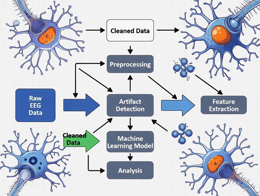
Experimental Workflows and Signaling Pathways
EEG Artifact Removal and Analysis Workflow
ICA-Based Artifact Separation Principle
FAQ: Understanding and Identifying Physiological Artifacts
Q1: What are physiological artifacts, and why are they a critical issue in EEG research? Physiological artifacts are unwanted signals in EEG recordings that originate from the body's own non-neural activities, such as eye movements, muscle contractions, or heartbeats [1] [8]. They are a primary concern because their amplitude is often much larger than neural signals, potentially masking brain activity, biasing analysis, and leading to misinterpretation or clinical misdiagnosis [1] [8]. Accurately identifying and removing them is a foundational step for ensuring data integrity in neuroscience research and drug development.
Q2: How can I distinguish between common physiological artifacts based on their appearance? Each major physiological artifact has a characteristic signature in the time and frequency domains. The table below summarizes key identifying features.
Table: Identification Guide for Common Physiological Artifacts
| Artifact Type | Origin | Time-Domain Effect | Frequency-Domain Effect | Most Affected Channels |
|---|---|---|---|---|
| Ocular (EOG) | Corneo-retinal dipole (eye blinks, movements) [8] | Sharp, high-amplitude deflections [8] | Dominant in low frequencies (Delta, Theta bands) [8] | Frontal (e.g., Fp1, Fp2) [8] |
| Muscle (EMG) | Muscle contractions (jaw, neck, face) [1] [8] | High-frequency, chaotic "noise" [1] | Broadband, dominates Beta/Gamma bands (>13 Hz) [8] | Temporal, Frontotemporal [9] |
| Cardiac (ECG) | Electrical activity of the heart [1] [10] | Rhythmic, recurring waveform (pulse artifact) [10] | Overlaps multiple EEG bands; fundamental at heart rate [10] | Central, neck-adjacent channels [8] |
| Sweat | Low-frequency shifts from sweat glands [8] | Very slow, large baseline drifts [8] | Contaminates Delta and Theta bands [8] | Widespread, often all channels [8] |
Q3: My analysis pipeline is automated. Are there quantitative detection methods I can use? Yes, several automated methods leverage statistical and spectral properties of the signal for detection [9]. These are often applied after a decomposition technique like Independent Component Analysis (ICA) to increase sensitivity [9].
Table: Quantitative Methods for Automated Artifact Detection
| Detection Method | Primary Principle | Best For Identifying |
|---|---|---|
| Spectral Thresholding | Identifies power exceeding a threshold in specific frequency bands [9] | Muscle (20-60 Hz), Ocular (1-3 Hz) artifacts [9] |
| Extreme Value | Flags data points exceeding a fixed voltage threshold [9] | Gross ocular artifacts and large movement transients [9] |
| Kurtosis | Measures how "peaked" or outlier-heavy the data distribution is [9] | Components with transient, high-amplitude peaks (e.g., eye blinks) [9] |
| Joint-Probability | Calculates the improbability of a data sample given the overall distribution [9] | Unusual or transient events that are statistical outliers [9] |
Troubleshooting Guides
Issue 1: Persistent Ocular Artifacts Overwhelming Frontal Channels
Problem: Eye blinks and movements create large, recurring deflections in frontal EEG channels, obscuring cognitive signals of interest.
Solution:
- Pre-processing: Apply a high-pass filter with a cutoff of 0.5-1.0 Hz can reduce slow drifts from eye movements, but use caution as it may also distort neural data [11].
- Advanced Correction: Use Independent Component Analysis (ICA) to separate and remove artifact components [3] [9]. This is the most common and effective method.
- Workflow: After standard filtering and epoching, run ICA on your data.
- Identification: Correlate independent components with a recorded EOG channel or visually inspect components for a frontal scalp topography and time course linked to blinks [9].
- Removal: Subtract the identified artifact components from the data.
- Experimental Control: Instruct participants to fixate on a point and minimize blinks during critical trial periods, if the protocol allows.
Issue 2: Contamination from Muscle Activity (EMG) in Temporal Regions
Problem: High-frequency noise from jaw clenching, swallowing, or neck tension contaminates temporal channels, masking beta and gamma brain oscillations.
Solution:
- Spectral Analysis: Inspect the power spectrum of suspicious channels for elevated power in the 20-60 Hz range [9].
- ICA-Based Removal: ICA can effectively separate and remove muscle artifacts, as they are statistically independent from brain signals [3] [1].
- Alternative Methods: For wearable EEG with low channel counts, consider deep learning approaches (e.g., CNN-LSTM models) or ASR-based pipelines, which are emerging as powerful tools for muscular and motion artifacts [3] [12] [8].
- Protocol Adjustment: Ensure participants are relaxed and remind them to unclench their jaw and relax their face during recording.
Issue 3: Rhythmic Cardiac Artifact Mimicking Neural Activity
Problem: The QRS complex from the heartbeat appears as a rhythmic artifact in central or neck-adjacent EEG channels [10] [8].
Solution:
- Detection: Use an R-peak detection algorithm (e.g.,
R_peak_detect.min MATLAB) on a simultaneously recorded ECG channel or an EEG channel showing the clearest artifact [10]. - Targeted Filtering: Instead of filtering the entire signal, apply a zero-phase filter only to the EEG segments time-locked to the detected QRS complexes. This preserves neural information outside of these brief windows [10].
- Component-Based Removal: ICA can also be used to isolate and remove cardiac components, which have a stable, periodic time course and a characteristic topography [1] [9].
Issue 4: Slow Baseline Drifts Caused by Perspiration
Problem: Slow, large-amplitude drifts in the signal caused by sweat, which can saturate amplifiers and distort event-related potentials.
Solution:
- Filtering: A high-pass filter with a very low cutoff (e.g., 0.1 Hz or 0.5 Hz) is often effective at removing these slow drifts [8].
- Linear Detrending: For shorter epochs, applying linear detrending can help remove slow, linear shifts in the baseline [11].
- Environmental Control: Record in a cool, temperature-controlled environment to minimize sweating.
Experimental Protocols for Artifact Management
Protocol 1: Ocular Artifact Removal Using Independent Component Analysis (ICA)
This is a widely adopted methodology for correcting eye blinks and movements [3] [9].
Workflow Overview:
Detailed Methodology:
- Preprocessing: Begin with raw, continuous EEG data. Apply a 1 Hz high-pass filter to remove slow drifts that can impede ICA performance.
- Epoching: Segment the data into epochs (e.g., -100 ms to 600 ms around a stimulus) if analyzing event-related potentials.
- ICA Decomposition: Use an ICA algorithm (e.g., Infomax, FastICA) to decompose the epoched data into independent components. Each component consists of a fixed scalp topography and an associated time course [9].
- Component Identification: Identify components representing ocular artifacts. Key indicators include:
- A scalp topography showing strong, focal projections to frontal electrodes.
- A time course containing large, infrequent deflections that correlate with known blink events or a recorded EOG channel [9].
- Artifact Removal & Reconstruction: Subtract the identified artifact components from the data. The remaining components are then back-projected to the sensor space to create the cleaned EEG dataset.
Protocol 2: Targeted Cardiac Artifact Removal via QRS Detection
This protocol is effective for removing pulse artifacts without distorting the entire EEG signal [10].
Workflow Overview:
Detailed Methodology:
- Data Acquisition: Record a simultaneous ECG signal alongside the EEG.
- R-Peak Detection: Use an algorithm (e.g., the open-source
R_peak_detect.mfunction for MATLAB) to accurately identify the R-peaks of the QRS complex in the ECG signal [10]. - Epoch Definition: Define short time windows around each detected R-peak that encompass the entire QRS complex.
- Targeted Filtering: Apply a zero-phase filter only to these short EEG segments that are time-locked to the cardiac cycle. This method prevents the loss of important neural information in the rest of the signal that would occur if the entire dataset were filtered [10].
The Scientist's Toolkit: Research Reagent Solutions
Table: Essential Tools and Algorithms for Physiological Artifact Management
| Tool/Algorithm | Function | Application Notes |
|---|---|---|
| Independent Component Analysis (ICA) | Blind source separation; decomposes EEG into independent components for artifact identification and removal [3] [1] [9]. | Gold standard for ocular and cardiac artifacts. Less effective for non-stationary muscle noise. Requires multi-channel data. |
| Automated Spike Detection (e.g., Autoreject) | Automatically detects and rejects bad trials or channels based on statistical thresholds [11]. | Useful for initial data cleaning. May reject useful data if not calibrated carefully. |
| Wavelet Transform | Time-frequency analysis that allows for localized denoising of specific artifact components [3] [1]. | Effective for non-stationary artifacts like EMG. Can be combined with other methods in hybrid pipelines. |
| Deep Learning Models (e.g., CNN-LSTM, GANs) | Learns complex patterns to separate clean EEG from artifacts in an end-to-end manner [3] [12]. | Emerging, powerful approach; promising for real-time applications and motion artifacts. Requires large datasets for training. |
| Artifact Subspace Reconstruction (ASR) | Statistical method that removes high-variance components in sliding windows [3]. | Widely applied for ocular, movement, and instrumental artifacts in wearable EEG. |
| Zero-Phase Filtering | Filters data in forward and reverse directions to eliminate phase distortion [10]. | Crucial for targeted filtering (e.g., cardiac artifact removal) to preserve temporal relationships. |
Troubleshooting Guides
Power Line Interference (Mains Noise)
Problem: High-frequency, monotonous noise at 50 Hz or 60 Hz is present across many or all channels, often obscuring the neural signal of interest. This interference originates from electromagnetic fields generated by alternating current (AC) in power lines and electronic equipment [13] [14].
Identification:
- Visual Pattern: Rhythmic, high-frequency oscillations that are very regular in appearance [15] [14].
- Spectral Profile: A sharp peak at exactly 50 Hz (e.g., in Europe) or 60 Hz (e.g., in the USA) in the frequency spectrum [13] [16].
Solutions:
| Troubleshooting Step | Description | Rationale |
|---|---|---|
| Preventive Measures | Use actively shielded cables and keep them short. Remove unnecessary electronics from the recording environment. Ensure the recording room is properly grounded [14] [17]. | Active shielding minimizes capacitive coupling from AC fields. Short cables reduce the antenna effect [14]. |
| Notch Filtering | Apply a notch filter at 50 Hz or 60 Hz during post-processing [13] [14]. | This directly attenuates power at the specific interference frequency. Caution is advised as it can cause signal distortions and ringing artifacts in the time domain [16]. |
| Advanced Processing | Use modern denoising algorithms like Spectrum Interpolation, CleanLine, or Discrete Fourier Transform (DFT) filtering [16]. | These methods can remove line noise with less signal distortion compared to traditional notch filters, especially when noise amplitude fluctuates [16]. |
Electrode Pop
Problem: A single channel shows a sudden, large, steep deflection (positive or negative) that quickly returns to baseline. This is caused by a sudden change in impedance at the electrode-skin interface [13] [18].
Identification:
- Visual Pattern: A single channel shows a sudden, large, steep deflection (positive or negative) that quickly returns to baseline. The artifact has no electrical field, meaning it is confined to one electrode [15] [18].
- Common Causes: A loose or drying electrode; poor initial contact; pressure or pull on the electrode cable; a dirty electrode [14] [18].
Solutions:
| Troubleshooting Step | Description | Rationale |
|---|---|---|
| Preventive Measures | Ensure all electrodes are firmly attached with good conductive contact before starting the recording. Check impedances to identify poor connections [14] [17]. | A stable, low-impedance connection prevents sudden shifts in conductivity that cause pops [13]. |
| Immediate Action | If pops occur during a recording, check and re-attach the offending electrode. Visually inspect for dried gel or physical displacement [18]. | Fixing the physical connection problem is the most direct solution. |
| Post-Processing | Mark the affected channel segment for rejection. For persistently bad channels, consider replacing (interpolating) the entire channel's data using signals from surrounding good channels [13] [17]. | This prevents the large, non-physiological spike from contaminating the analysis. Interpolation should be used cautiously [13]. |
Cable Movement
Problem: Sudden, high-amplitude, irregular deflections appear in the data, often correlated with participant movement. This is caused by triboelectric noise (friction within the cable) or conductor motion in a magnetic field [13] [14].
Identification:
- Visual Pattern: Sudden, high-amplitude, irregular deflections in the signal [14]. If the cable swings rhythmically, it may induce oscillations at the swing frequency [13].
- Context: The artifact is directly correlated with participant movement [13].
Solutions:
| Troubleshooting Step | Description | Rationale |
|---|---|---|
| Preventive Measures | Use high-quality, low-noise cables with active shielding. Secure cables to the participant's body or cap using Velcro or tape to minimize movement [14] [17]. | Active shielding eliminates capacitive coupling, and securing cables reduces triboelectric noise and physical strain [14]. |
| Hardware Setup | In wireless systems, ensure the transmitter is securely fixed to the cap. Keep cable lengths as short as practically possible [17]. | Minimizing moving parts and cable length directly reduces the source of the artifact [17]. |
| Post-Processing | Identify and mark movement-corrupted segments for artifact rejection. Filtering may attenuate slow drifts from cable sway, but overlapping artifacts are hard to separate from neural data [13]. | This excludes sections of data where the signal is irrevocably contaminated by motion [13]. |
Frequently Asked Questions (FAQs)
Q1: Why should I avoid using a notch filter as my first choice for removing power line noise? While effective at removing noise at a specific frequency, notch filters (especially IIR filters like Butterworth) can introduce ringing artifacts and distort the time-domain signal, which is critical for analyzing event-related potentials (ERPs) [16]. It is often preferable to use methods like Spectrum Interpolation or CleanLine, which have been shown to remove non-stationary line noise with less distortion [16].
Q2: My reference electrode has a poor connection. How does this affect my data? The reference electrode is crucial as it provides the baseline against which all other electrodes are measured. A bad reference connection will introduce artifacts into every single channel of your recording if you are using a common reference montage [14] [17]. Always ensure your reference electrode has a stable, low-impedance connection.
Q3: Can I use deep learning to remove these artifacts? Yes, deep learning is an emerging and powerful tool for EEG artifact removal. Models like Generative Adversarial Networks (GANs), sometimes combined with Long Short-Term Memory (LSTM) networks, are being developed to effectively separate artifacts from neural signals while preserving the underlying brain activity [12]. These methods can learn complex patterns and show promising results in handling various artifact types.
Q4: One of my electrodes keeps popping. I've re-applied it, but the problem continues. What should I do? First, check the cable and connector for damage. If the hardware is intact, the issue may be persistent poor contact or drying gel. Your best options are to:
- Re-reference your data to a different, stable electrode (e.g., from the left to the right mastoid) if your montage allows [18].
- Exclude the bad channel from analysis and, for high-density arrays, interpolate its data from neighboring good channels [13].
Table 1: Performance Comparison of Power Line Noise Removal Methods [16]
| Method | Key Principle | Advantages | Disadvantages |
|---|---|---|---|
| Notch Filter | Bandstop filter attenuating a narrow frequency band. | Simple and widely available. | Can cause severe ringing artifacts and signal distortion in the time domain [16]. |
| DFT Filter | Fits and subtracts sine/cosine waves at the noise frequency. | Avoids corrupting frequencies away from the line noise. | Assumes constant noise amplitude; fails with fluctuating noise [16]. |
| CleanLine | Regression-based approach using multitapers. | Removes only deterministic line components, preserving background spectrum. | May fail with large, non-stationary artifacts [16]. |
| Spectrum Interpolation | Interpolates the noise frequency in the Fourier spectrum. | Less signal distortion than a notch filter; handles non-stationary noise well. | Requires transformation to frequency domain and back [16]. |
Table 2: Essential Research Reagent Solutions & Materials
| Item | Function in Artifact Mitigation |
|---|---|
| Active Electrode Systems | Amplify the signal at the electrode source, making it more resilient to cable movement and environmental interference [13] [14]. |
| Low-Noise, Actively Shielded Cables | Minimize the pickup of mains interference and reduce triboelectric noise caused by cable movement [14]. |
| High-Quality Electrolyte Gel | Ensures stable, low-impedance contact between electrode and skin, preventing electrode pops and slow drifts [17]. |
| Faraday Cage / Shielded Room | Electromagnetically isolates the recording setup, physically blocking external noise sources [17]. |
Experimental Protocols
Protocol: Removing Power Line Noise via Spectrum Interpolation
This protocol is adapted from methods shown to effectively remove non-stationary power line noise with minimal distortion [16].
- Data Segmentation: Divide the continuous EEG data into manageable, possibly overlapping, segments (e.g., 1-2 seconds in length).
- Fourier Transform: Apply a Discrete Fourier Transform (DFT) to each segment to convert the data from the time domain to the frequency domain.
- Identify and Interpolate: In the amplitude spectrum, identify the bin(s) corresponding to the power line frequency (e.g., 50 Hz) and its harmonics.
- Interpolate: Replace the amplitude values at these bins by interpolating from the neighboring frequency bins on either side. A linear or spline interpolation can be used.
- Inverse Transform: Apply an Inverse Discrete Fourier Transform (iDFT) to reconstruct the time-domain signal without the targeted line noise components.
Protocol: A Multi-Channel Wiener Filter for Stimulation Artifact Removal
This advanced protocol uses a linear Wiener filter to predict and remove large artifacts caused by electrical stimulation, which is common in neural implant and BCI research [19].
- Record Stimulation Input and Artifact Output: Apply a known, varying electrical stimulation current (the input signal, x[n]) while recording the resulting large artifacts (the output signal, y[m]) on all recording channels in the absence of neural activity.
- Calculate Correlation Matrices: Compute the covariance matrix of the input signals (Cxx) and the cross-correlation matrix between the output and input signals (Ryx).
- Estimate Wiener Filter: Calculate the optimal multi-channel Wiener filter (ĥ) that maps the stimulation currents to the recorded artifacts using the Wiener-Hopf equation: ĥ = (Cxx)⁻¹Ryx.
- Apply Filter for Prediction: During the actual experiment with concurrent neural activity, use the derived filter (ĥ) to predict the artifact on each recording channel by convolving the stimulation current with the filter.
- Subtract Prediction: Subtract the predicted artifact from the recorded signal to reveal the underlying neural activity.
FAQ: Understanding EEG Artifacts and Their Consequences
What is an EEG artifact and why is it a problem? An EEG artifact is any signal recorded by the EEG that does not originate from the brain's electrical activity [20] [8]. These unwanted signals contaminate the recording, obscuring genuine neural information. Because EEG measures very weak signals in the microvolt range, artifacts can easily mimic or mask true brain activity, leading to incorrect data interpretation and potentially severe clinical misdiagnosis, such as confusing an artifact with epileptiform activity [8].
What are the most common types of artifacts I might encounter? Artifacts are typically categorized by their origin. The table below summarizes the primary types, their causes, and their impact on the EEG signal [1] [13] [8].
Table 1: Common EEG Artifacts and Their Characteristics
| Artifact Type | Origin/Cause | Key Characteristics | Impact on EEG Signal |
|---|---|---|---|
| Ocular (EOG) | Eye blinks and movements [13] [8]. | Slow, high-amplitude deflections; most prominent over frontal electrodes [13]. | Obscures frontal delta/theta rhythms; can mimic cognitive processes [8]. |
| Muscle (EMG) | Head, jaw, or neck muscle contractions (e.g., clenching, talking) [13] [8]. | High-frequency, broadband noise; "spiky" morphology in time domain [13]. | Masks beta/gamma band activity; reduces clarity across entire spectrum [8]. |
| Cardiac (ECG/Pulse) | Electrical activity of the heart or pulse-induced electrode movement [13] [8]. | Rhythmic, recurring waveform synchronized with the heartbeat [13]. | Can be mistaken for a cerebral rhythm or epileptiform discharge [13]. |
| Electrode Pop | Sudden change in electrode-skin impedance (e.g., from drying gel) [13] [8]. | Very sharp, high-amplitude transient typically isolated to a single channel [13]. | Introduces large, non-physiological spikes that can be misinterpreted as pathological [8]. |
| Line Noise | Electromagnetic interference from AC power (50/60 Hz) [13] [8]. | Persistent high-frequency oscillation at 50 or 60 Hz [13]. | Obscures high-frequency neural oscillations and adds non-neural noise [8]. |
How can artifacts directly lead to misdiagnosis? Artifacts pose a direct risk to patient safety by mimicking genuine neurological phenomena. For instance [8]:
- A muscle artifact from head or neck tension can be misinterpreted as an epileptic spike or seizure activity.
- A pulse artifact, caused by the rhythmic movement of an electrode near a blood vessel, can resemble a cerebral rhythm or periodic discharge, potentially leading to an incorrect diagnosis of epilepsy [13]. The core challenge is that artifacts do not conform to a realistic head model of brain activity, but their appearance can be deceptively similar to real abnormalities [20].
What is the foundational concept for recognizing an artifact? The primary foundation for recognizing artifacts is identifying the mismatch between potentials generated by the brain and activity that does not conform to a realistic head model [20]. This involves assessing whether the signal's spatial distribution, frequency content, and timing are physiologically plausible for neural origins.
Troubleshooting Guides: Artifact Identification and Removal
Guide 1: Identifying Common Artifacts in Your Recording
Use this workflow as a decision tree to identify unknown artifacts in your EEG data. The diagram below outlines the logical steps for diagnosing common artifact types based on their visual characteristics.
Guide 2: Selecting an Artifact Removal Method
No single artifact removal method is optimal for all situations. The choice depends on the artifact type, analysis requirements, and available resources. The following table compares the most prevalent techniques used in the field [1] [21].
Table 2: Comparison of Prevalent EEG Artifact Removal Methods
| Method | Best For | Key Advantages | Key Limitations | Suitability for Online Use |
|---|---|---|---|---|
| Independent Component Analysis (ICA) | Ocular and large muscle artifacts [1] [13]. | Does not require reference channels; effective for separating sources [1]. | Requires multi-channel data; computationally intensive; manual component selection can be subjective [21]. | Limited [21]. |
| Regression (in Time/Frequency Domain) | Ocular artifacts when EOG reference is available [1]. | Simple principle and implementation [1]. | Requires reference channels (EOG); can lead to over-correction and removal of neural signals [1] [21]. | Possible [21]. |
| Wavelet Transform | Non-stationary artifacts like EMG and electrode pops [1]. | Good for analyzing transient signals and local features in time and frequency [1]. | Parameter selection (e.g., mother wavelet) can be complex; can alter the underlying EEG [21]. | Possible [21]. |
| Deep Learning (e.g., AnEEG, GANs) | Complex artifacts in high-density EEG; automated pipelines [12]. | High performance; can model complex patterns; potential for full automation [12]. | Requires large datasets for training; "black-box" nature reduces interpretability [22] [12]. | Yes (with pre-trained models) [12]. |
| Blind Source Separation (BSS) | Various artifacts, especially when reference channels are unavailable [1]. | Does not require reference channels; versatile [1]. | Can be computationally complex; may not separate all artifacts perfectly [1] [21]. | Limited [21]. |
The diagram below provides a structured workflow for selecting the most appropriate artifact removal strategy based on your specific context and constraints.
Guide 3: Experimental Protocol for Deep Learning-Based Artifact Removal
The following protocol outlines the methodology for implementing a deep learning-based artifact removal tool, such as the AnEEG model, which uses a Generative Adversarial Network (GAN) with LSTM layers [12].
Objective: To remove multiple types of artifacts from EEG signals while preserving the underlying neural information. Key Components of the AnEEG Model [12]:
- Generator: A network that takes artifact-contaminated EEG as input and generates cleaned EEG as output. It typically uses LSTM layers to capture temporal dependencies in the signal.
- Discriminator: A network that judges whether the signal produced by the Generator is "clean" (i.e., indistinguishable from a ground-truth clean EEG) or artificially generated.
- Adversarial Training: The Generator and Discriminator are trained simultaneously in a competitive process, where the Generator strives to produce cleaner signals, and the Discriminator becomes better at detecting artifacts, leading to overall improvement.
Procedure:
- Data Preparation:
- Acquire EEG datasets containing both artifact-contaminated signals and corresponding ground-truth clean signals. These can be semi-simulated (by linearly mixing clean EEG with EOG/EMG) or real datasets with clean segments identified by experts [12].
- Preprocess the data (e.g., band-pass filtering, normalization) and segment it into epochs.
- Split the data into training, validation, and test sets.
Model Training:
- Train the GAN model on the contaminated EEG inputs with the goal of producing outputs that match the clean EEG targets.
- The loss function typically combines:
- Adversarial Loss: Measures the Discriminator's ability to distinguish real from generated signals.
- Content Loss (e.g., L1 or L2 loss): Ensures the generated signal is structurally similar to the ground-truth clean signal [12].
Model Validation & Testing:
- Validate the model on a separate dataset using quantitative metrics (see below).
- Test the final model on a held-out test set to evaluate its performance.
Performance Metrics for Validation [12]:
- NMSE (Normalized Mean Square Error): Lower values indicate better agreement with the original signal.
- CC (Correlation Coefficient): Higher values mean a stronger linear relationship with the ground truth.
- SNR (Signal-to-Noise Ratio) & SAR (Signal-to-Artifact Ratio): Higher values indicate better artifact suppression.
The Scientist's Toolkit: Key Research Reagents & Solutions
This table details essential materials and computational tools referenced in the featured experiment and broader field of EEG artifact research [12] [23].
Table 3: Essential Research Tools for Advanced EEG Artifact Handling
| Tool / Reagent | Function / Description | Application Context |
|---|---|---|
| GAN with LSTM (AnEEG) | A deep learning architecture for generating artifact-free EEG signals from noisy inputs [12]. | Automated, high-performance artifact removal for standard EEG [12]. |
| TMS-Compatible EEG Amplifier | A specialized amplifier designed to handle the massive voltage spike induced by a TMS pulse without saturating [23]. | Essential for clean data acquisition in combined TMS-EEG studies [23]. |
| Carbon-Wire Loops (CWL) | Reference sensors placed on the head that exclusively capture MR-induced artifacts without neural signals [24]. | Critical for effective artifact removal in simultaneous EEG-fMRI recordings [24]. |
| Reference EOG/ECG Electrodes | Additional electrodes placed to specifically record eye movement and heart activity [1]. | Provides a reference signal for regression-based removal of ocular and cardiac artifacts [1] [21]. |
| ICA Algorithm (e.g., in EEGLAB) | A blind source separation algorithm that decomposes multi-channel EEG into independent components for manual or automatic artifact rejection [1] [13]. | Versatile tool for analyzing and removing various artifacts from standard EEG recordings [1]. |
Simultaneous Electroencephalography and functional Magnetic Resonance Imaging (EEG-fMRI) is a powerful multimodal technique that combines the high temporal resolution of EEG with the high spatial resolution of fMRI, providing unparalleled insights into brain dynamics. However, EEG signals recorded inside an MRI scanner are contaminated by severe artifacts that can be hundreds of times greater than the neural signals of interest. These artifacts originate from the MRI environment itself and pose significant challenges for researchers and clinicians. The three primary artifacts are gradient artifacts caused by switching magnetic field gradients during image acquisition, ballistocardiogram (BCG) artifacts resulting from cardiac-related movements in the static magnetic field, and motion artifacts from subject movement. Effective management of these artifacts is essential for obtaining reliable neural data and accurate interpretation of brain connectivity and function. This technical support center provides comprehensive troubleshooting guides and FAQs to address the specific issues researchers encounter during simultaneous EEG-fMRI experiments.
Frequently Asked Questions (FAQs)
What are the main types of artifacts in simultaneous EEG-fMRI?
- Gradient Artifacts (GA): These are the largest source of noise, induced by the rapid switching of magnetic field gradients during fMRI acquisition. The amplitude of GAs can be up to 100 times greater than the EEG signal and their frequency content overlaps with that of neural signals, making simple filtering ineffective [25] [26].
- Ballistocardiogram (BCG) Artifacts: These are caused by cardiac-related head and body movements, as well as the pulsatile flow of blood (a conductive fluid) in the static magnetic field. The BCG artifact is time-locked to the heartbeat and can have an amplitude 3-4 times that of the EEG signal [25] [26] [27].
- Motion Artifacts: These occur when the subject's head moves within the scanner, inducing currents in the EEG electrodes according to Faraday's law of induction. This movement can be caused by the subject themselves or by cardio-balistic forces [25].
- Environmental Artifacts: This category includes interference from power lines, ventilation systems, lights in the MR room, and vibrations from the scanner's helium cooling pump [25].
Which BCG artifact removal method should I choose for my study?
The choice of method depends on your analysis goals, as different methods have distinct strengths and weaknesses. The table below summarizes the performance characteristics of common BCG artifact removal techniques, based on a 2025 systematic evaluation [28].
Table 1: Performance Comparison of BCG Artifact Removal Methods
| Method | Best Performance Metric | Key Characteristic | Impact on Network Topology |
|---|---|---|---|
| Average Artifact Subtraction (AAS) | Best signal fidelity (MSE = 0.0038, PSNR = 26.34 dB) [28] | Template-based subtraction; simple but can leave residuals [28] [25] | Affects functional connectivity patterns [28] |
| Optimal Basis Set (OBS) | Highest structural similarity (SSIM = 0.72) [28] | Uses PCA to capture artifact variations; better for temporal structure [28] [26] | Significantly affects network structure [28] |
| Independent Component Analysis (ICA) | Greater sensitivity in dynamic graph metrics [28] | Blind source separation; requires manual component selection [28] [25] | Shows frequency-specific patterns in dynamic graphs [28] |
| OBS + ICA (Hybrid) | Lowest p-values in dynamic connectivity (e.g., theta-beta bands) [28] | Combines strengths of OBS and ICA [28] [27] | Reveals pronounced frequency-specific effects [28] |
| Denoising Autoencoder (DAR) | High SSIM (0.8885) and SNR gain (14.63 dB) [29] [30] | Deep learning approach; learns direct mapping from noisy to clean signals [29] [30] | Not fully characterized for network topology [29] |
For signal quality, AAS or the deep learning-based DAR are strong candidates. If your focus is functional connectivity or network analysis, OBS or hybrid methods (e.g., OBS+ICA) may be more appropriate, as they better preserve the relationships between signals. ICA, while sometimes weaker on pure signal metrics, can be valuable for detecting frequency-specific patterns in dynamic analyses [28].
Can I use simultaneous EEG-fMRI for real-time applications like neurofeedback?
Yes, recent advances have made real-time artifact removal feasible. The EEG-LLAMAS platform is an open-source software specifically designed for low-latency BCG artifact removal. It has been validated for real-time use, introducing an average lag of less than 50 ms, which makes it suitable for closed-loop neurofeedback paradigms within the MRI environment [31] [32].
Why does my EEG data still contain artifacts after applying AAS?
Residual artifacts after Average Artifact Subtraction are common and are often due to temporal jitter. This jitter arises because the MRI machine and the EEG system typically operate on separate clocks, causing slight variations in the sampling of each artifact instance. This in turn degrades the accuracy of the averaged template [26]. To mitigate this, ensure your setup uses synchronized clocks between the EEG and MRI systems. Alternatively, consider using methods like the Optimal Basis Set (OBS) or FASTR, which are explicitly designed to account for this variability by modeling the principal components of the artifact residuals [26].
How do I effectively remove Gradient Artifacts?
The FASTR algorithm, an advanced form of OBS, is widely considered effective for gradient artifact removal. Unlike simple AAS, which uses one average template, FASTR constructs a unique artifact template for each slice in each EEG channel. It then supplements the average with a linear combination of basis functions derived from PCA on the artifact residuals, leading to more thorough cleanup [26]. Furthermore, the choice of fMRI sequence matters. Spiral sequences generate gradient artifacts an order of magnitude larger than Echo Planar Imaging (EPI) sequences. However, with accurate synchronization, AAS can suppress artifacts from both sequences effectively below 80 Hz [33].
Troubleshooting Guides
Guide 1: Systematic Artifact Removal Workflow
The following diagram provides a logical workflow for tackling artifacts in your EEG-fMRI data.
Guide 2: Addressing Poor BCG Artifact Removal
If BCG artifact removal is unsatisfactory, follow this troubleshooting guide.
Experimental Protocols for Key Artifact Removal Methods
Protocol 1: Optimal Basis Set (OBS) for BCG and Gradient Artifacts
The OBS method improves upon AAS by accounting for variability in the artifact shape over time [26].
- Artifact Epoching: Segment the continuous EEG data into epochs time-locked to each heartbeat (for BCG) or slice trigger (for gradient artifacts).
- Template Creation: Compute an average artifact template for each channel from the epochs.
- Principal Component Analysis (PCA): Perform PCA on the matrix of artifact epochs. The dominant principal components form the "Optimal Basis Set" that captures the main modes of artifact variation.
- Projection and Subtraction: For each artifact epoch, project it onto the optimal basis set to create a patient- and time-specific template.
- Subtraction: Subtract this tailored template from the original EEG signal in each epoch.
- Signal Reconstruction: Reconstruct the continuous, cleaned EEG signal from the processed epochs.
Protocol 2: Hybrid OBS-ICA Method
This protocol combines the template-based approach of OBS with the blind source separation of ICA, often yielding superior results for connectivity analysis [28] [27].
- Apply OBS: First, clean the data using the standard OBS protocol (steps 1-6 above). This will remove the bulk of the BCG artifact but may leave some residuals.
- Apply ICA: Perform Independent Component Analysis (e.g., using Infomax or FastICA algorithms) on the OBS-cleaned data.
- Component Identification: Manually inspect the resulting independent components and their topographies to identify any residual artifact components. These often have a stereotypical BCG shape or a non-brain-like topography.
- Component Removal: Remove the identified artifact components.
- Signal Reconstruction: Project the remaining components back to the sensor space to obtain the final cleaned EEG signal.
The following tables consolidate key performance metrics from recent studies to aid in method selection.
Table 2: Quantitative Performance of Artifact Removal Methods
| Method | Key Metric | Reported Value | Context / Frequency Band |
|---|---|---|---|
| AAS | Mean Squared Error (MSE) | 0.0038 [28] | Best performance for signal fidelity [28] |
| AAS | Peak Signal-to-Noise Ratio (PSNR) | 26.34 dB [28] | Best performance for signal fidelity [28] |
| OBS | Structural Similarity Index (SSIM) | 0.72 [28] | Best performance for structural similarity [28] |
| DAR (Deep Learning) | Root-Mean-Squared Error (RMSE) | 0.0218 ± 0.0152 [29] [30] | Outperforms traditional methods [29] |
| DAR (Deep Learning) | Structural Similarity Index (SSIM) | 0.8885 ± 0.0913 [29] [30] | Outperforms traditional methods [29] |
| DAR (Deep Learning) | SNR Gain | 14.63 dB [29] [30] | Significant improvement over noisy input [29] |
Table 3: Impact on Functional Connectivity (Graph Theory Metrics)
| Artifact Removal Method | Impact on Dynamic Connectivity | Notable Frequency Band Effects |
|---|---|---|
| AAS | Method-specific differences observed [28] | Affects network topology across bands [28] |
| OBS | Method-specific differences observed [28] | Affects network topology across bands [28] |
| ICA | Greater sensitivity in dynamic graphs [28] | Reveals frequency-specific patterns [28] |
| OBS + ICA | Lowest p-values across frequency pairs [28] | Pronounced effects in theta-beta & delta-gamma pairs [28] |
| All Methods | Dynamic analysis shows more pronounced effects than static analysis [28] | Beta and gamma bands show stronger differentiation [28] |
The Scientist's Toolkit: Research Reagent Solutions
Table 4: Essential Hardware and Software for EEG-fMRI Artifact Management
| Item | Type | Function / Application |
|---|---|---|
| MRI-Compatible EEG Amplifier | Hardware | Essential for safe operation inside the scanner; resistant to electromagnetic interference. |
| Synchronization Interface | Hardware | Synchronizes the EEG and MRI clocks to reduce temporal jitter in gradient artifacts [26] [33]. |
| Reference Layer / Carbon Wire Loops | Hardware | Active hardware solution that records artifact signals from a separate layer for subtraction, significantly reducing BCG artifacts [27]. |
| Piezoelectric Sensor / ECG Electrodes | Hardware | Provides a precise reference signal of cardiac activity (QRS complex) for BCG artifact removal algorithms [26]. |
| EEG-LLAMAS Software | Software | Open-source platform for real-time, low-latency (<50 ms) BCG artifact removal, enabling neurofeedback [31]. |
| FASTR Algorithm | Software | An advanced OBS method implemented in software (e.g., in FMRIB's EEGLAB plugin) for effective gradient and BCG artifact removal [26]. |
| Denoising Autoencoder (DAR) | Software (Algorithm) | A deep learning framework that learns to map artifact-contaminated EEG to clean signals, showing state-of-the-art performance [29] [30]. |
From Theory to Practice: A Survey of Modern EEG Artifact Removal Techniques
FAQ: System Setup and Selection
What are the key advantages of modern dry electrode systems over traditional gel-based electrodes? Dry electrode systems offer significant practical benefits for experimental setups. They eliminate the need for skin abrasion and conductive gel, reducing preparation time. Studies show the average setup time for dry electrodes is approximately 4 minutes, compared to over 6 minutes for wet systems [34]. Furthermore, dry electrodes maintain stable signal quality over longer recording periods because they avoid the signal degradation that occurs as conductive gel dries out [34]. Their design often includes features like ultra-high impedance amplifiers and mechanical isolation to stabilize against movement artifacts [34] [35].
My research involves movement. Should I choose a gel-based or dry EEG system? Dry EEG systems are often better suited for studies involving participant movement. While they can be more susceptible to motion artifacts due to the lack of a gel-based mechanical buffer, their shorter setup time and improved portability make them ideal for dynamic, real-world settings [35]. For the highest signal fidelity in a fully controlled, stationary environment, a gel-based system might still be preferable.
How scalable are modern EEG acquisition systems for high-throughput research? Modular acquisition systems based on Field-Programmable Gate Array (FPGA) technology now provide high scalability. You can start with a single, compact 8-lead acquisition module and use a daisy-chain interface to expand to 16 leads [36]. For even greater channel counts, multiple basic modules can be connected in parallel to a central FPGA unit, constructing a high-density, high-throughput system suitable for large-scale studies [36].
Troubleshooting Guides
Issue: Poor Signal Quality Across Multiple Channels
Symptoms: Unusually high impedance readings, signals appear noisy or flatlined across several channels.
Resolution Steps:
- Isolate the Problem: Follow the signal chain to identify the faulty component:
Recording Software -> Computer -> Amplifier -> Headbox -> Electrodes -> Participant[37]. - Check Electrode Connections: Ensure all electrodes are properly plugged in. Re-clean and re-apply electrodes, adding conductive gel or pressure as needed. Swap out electrodes to rule out a "dead" electrode [37].
- Test Hardware Components: Restart the recording software and amplifier. If the issue persists, try swapping the headbox with a known-working unit. If the problem disappears, the original headbox may be faulty [37].
- Investigate Participant-Specific Factors: If the issue remains after steps 1-3, the cause may be participant-specific. Remove all metal accessories from the participant. Check for hairstyle or skin products that might interfere. Try applying the ground electrode to a different location, such as the participant's hand or collarbone [37].
Issue: Persistent Artifacts in Dry EEG Recordings During Movement
Symptoms: Signal contains high-frequency noise or large amplitude shifts during participant movement.
Resolution Steps:
- Apply a Combined Cleaning Pipeline: Implement a multi-stage denoising strategy. A proven method involves first using ICA-based algorithms (like Fingerprint + ARCI) to remove physiological artifacts (eye, muscle, cardiac), followed by spatial filtering (like Spatial Harmonic Analysis - SPHARA) for general noise reduction [35].
- Validate with Quantitative Metrics: Assess the improvement by calculating standard deviation (SD), signal-to-noise ratio (SNR), and root mean square deviation (RMSD) pre- and post-processing. One study demonstrated that combining Fingerprint+ARCI with an improved SPHARA method reduced SD from 9.76 µV to 6.15 µV and improved SNR from 2.31 dB to 5.56 dB in dry EEG [35].
Performance Data for Hardware Selection
Table 1: Quantitative Comparison of EEG Artifact Removal Methods
| Method Category | Example Techniques | Key Performance Findings | Advantages | Limitations |
|---|---|---|---|---|
| Spatial & ICA-Based Combination | Fingerprint + ARCI + SPHARA [35] | Reduced SD to 6.15 µV; Improved SNR to 5.56 dB [35] | Effective for movement artifacts in dry EEG; complementary noise reduction. | Requires multi-step processing pipeline. |
| Advanced Deep Learning | CLEnet (Dual-scale CNN + LSTM) [38] | Achieved SNR of 11.50 dB and CC of 0.925 in mixed artifact removal [38] | End-to-end removal of multiple artifact types (EMG, EOG, ECG); suitable for multi-channel data. | Requires significant computational resources for training. |
| Generative Deep Learning | AnEEG (LSTM-based GAN) [12] | Lower NMSE/RMSE and higher CC vs. wavelet techniques [12] | Generates artifact-free signals; preserves original neural information. | Complex adversarial training process. |
Table 2: Technical Specifications of a Scalable EEG Acquisition Module
| Parameter | Specification | Research Implication |
|---|---|---|
| Core Chip | ADS1299 [36] | Provides high-quality acquisition with built-in pre-filtering and analog-to-digital conversion. |
| A/D Conversion | 24-bit [36] | Enables capture of microvolt-scale neural signals with high fidelity. |
| Sampling Rate | 250 - 4,000 SPS (for 8 leads) [36] | Offers flexibility for various paradigms, from slow cortical potentials to high-frequency activity. |
| Common-Mode Rejection | -110 dB [36] | Effectively suppresses ambient environmental noise. |
| Scalability | Daisy-chain stacking to 16 leads; parallel module connection [36] | Allows system to grow with research needs, from portable wearables to high-density setups. |
Experimental Protocols
Protocol 1: Validating a Combined Denoising Pipeline for Dry EEG
This protocol is designed to optimize artifact removal from dry EEG data collected during motor tasks [35].
Workflow: The experimental and data processing workflow is as follows:
Methodology Details:
- Equipment: 64-channel dry EEG cap with PU/Ag/AgCl electrodes [35].
- Paradigm: Use a motor execution task (e.g., left/right hand, feet, or tongue movements) with visual cues to generate reproducible cortical patterns [35].
- Processing - ICA-Based Cleaning: Apply the Fingerprint method to automatically identify and classify independent components containing physiological artifacts (ocular, muscular, cardiac). Follow this with the ARCI (Artifact Reconstruction and Subtraction using a Constrained ICA) algorithm to remove these artifacts [35].
- Processing - Spatial Denoising: Apply SPHARA, a spatial filter that uses the harmonic components of the sensor geometry to reduce noise while preserving neural signal patterns across the scalp [35].
- Validation: Calculate the following metrics on the processed data and compare them to the preprocessed (but uncleaned) signal to quantify improvement [35]:
- Standard Deviation (SD): Measures signal variability; lower values indicate reduced noise.
- Signal-to-Noise Ratio (SNR): Measures the level of the desired signal relative to background noise; higher values are better.
- Root Mean Square Deviation (RMSD): Quantifies the difference between the cleaned signal and a reference; interpretation is context-dependent.
Protocol 2: Implementing a Deep Learning-Based Artifact Removal Model
This protocol uses the CLEnet model for end-to-end removal of various artifacts from multi-channel EEG data [38].
Workflow: The deep learning pipeline for artifact removal involves the following stages:
Methodology Details:
- Model Architecture: CLEnet integrates two main branches [38]:
- Morphological Feature Extraction: Uses two Convolutional Neural Networks (CNNs) with different kernel sizes to identify and extract features at multiple scales. An improved one-dimensional Efficient Multi-Scale Attention (EMA-1D) module is embedded to enhance relevant temporal features during this process [38].
- Temporal Feature Extraction: Processes the features using a Long Short-Term Memory (LSTM) network to capture the temporal dependencies inherent in EEG signals [38].
- Training: The model is trained in a supervised manner using a mean squared error (MSE) loss function, which minimizes the difference between the model's output and the ground-truth clean EEG signals [38].
- Datasets: The model can be trained and validated on semi-synthetic datasets (where clean EEG is artificially mixed with EOG, EMG, or ECG) or on real datasets with labeled artifacts [38].
The Scientist's Toolkit
Table 3: Essential Research Reagents and Hardware for EEG Acquisition
| Item | Function / Explanation |
|---|---|
| Scalable EEG Acquisition Module | A foundational hardware unit, often based on chips like the ADS1299, that provides the core functions of signal amplification, filtering, and analog-to-digital conversion for a set number of channels. It forms the basis for scalable systems [36]. |
| FPGA (Field-Programmable Gate Array) Central Module | A reconfigurable hardware processor that enables high-throughput data streaming, parallel processing of multiple acquisition modules, and real-time implementation of complex algorithms like artifact removal [36]. |
| Dry PU/Ag/AgCl Electrodes | Dry-contact electrodes made from Polyurethane with Silver/Silver Chloride coating. They enable rapid setup without gel and are suitable for wearable systems, though may be more prone to movement artifacts [35]. |
| SPHARA (Spatial Harmonic Analysis) | A spatial filtering algorithm used for denoising. It leverages the geometric structure of the EEG electrode array to separate signal from noise in the spatial domain and is particularly effective when combined with other methods [35]. |
| ICA-Based Cleaning Algorithms (Fingerprint, ARCI) | A set of algorithms that use Independent Component Analysis to blindly separate recorded EEG into statistically independent components. These can be automatically or manually classified and removed before signal reconstruction [35]. |
| CLEnet Model | A pre-trained or customizable deep learning model integrating CNN and LSTM networks designed for end-to-end artifact removal from multi-channel EEG data, capable of handling multiple artifact types [38]. |
Troubleshooting Guides and FAQs for EEG Artifact Reduction
Frequently Asked Questions (FAQs)
Q1: What is the primary value of using ICA over simple artifact rejection for EEG data?
ICA allows for the subtraction of artifacts embedded in the data without removing the affected data portions. This is superior to simply rejecting bad data segments because it preserves the original amount of data, which leads to a higher signal-to-noise ratio for subsequent analysis. Artifact rejection, in contrast, reduces the number of trials available, which can be detrimental for analyses like multivariate pattern analysis that benefit from larger data sets [39] [40].
Q2: My ICA results look different each time I run it on the same data. Is this a problem?
Slight variations are normal. When using algorithms like Infomax ICA (runica), decompositions start with a random weight matrix, so convergence is slightly different every time [41]. Features that do not remain stable across multiple runs on the same data should not be interpreted. For a rigorous assessment of reliability, you can use tools like the RELICA plugin, which performs ICA on bootstrapped versions of your data [41].
Q3: How much data do I need to compute a stable ICA decomposition?
ICA works best with a large amount of basically similar and mostly clean data [41]. A general rule is that you need more than kN^2 data sample points, where N is the number of channels and k is a multiplier that tends to increase with the number of channels [42]. For example, with a 32-channel dataset, having 30,800 data points gives about 30 points per weight, which is sufficient. For high-density arrays (e.g., 256 channels), significantly more data is required [42].
Q4: What are the key criteria for identifying an artifact component versus a brain component?
You should evaluate multiple properties of each component [41]:
- Scalp Map: Artifacts have characteristic topographies. For example, eye blink components show strong frontal projections, while muscle artifacts can be more peripheral [41].
- Time Course: Inspect the component's activation for patterns like individual eye movements or high-frequency muscle noise [41].
- Power Spectrum: The power spectrum of an eye blink artifact typically shows a smoothly decreasing pattern, while muscle artifacts have broad-band high-frequency power [41].
- ERPimage: For epoched data, this can reveal if the component's activity is time-locked to events [41].
Q5: For single-channel EEG systems, can I still use ICA?
Standard multi-channel ICA is not applicable to single-channel data. However, alternative data-driven decomposition methods have been developed for single-channel EEG. These include techniques like Empirical Mode Decomposition (EMD), Singular Spectrum Analysis (SSA), and the more recent Fixed Frequency Empirical Wavelet Transform (FF-EWT), which can separate artifact sources from the single-channel signal [43].
Troubleshooting Common ICA Problems
Problem: Poor ICA Decomposition Quality
- Cause 1: Insufficient data. The dataset is too small for the number of channels.
- Solution: Ensure you have enough data points (see FAQ above). If data is limited, use the PCA option during ICA to reduce the number of components to be found [41].
- Cause 2: Presence of strong low-frequency drifts. Slow drifts reduce the independence of sources [44].
- Solution: Apply a high-pass filter before running ICA. A cutoff frequency of 1 Hz is recommended. Note that the ICA solution found from the filtered signal can be applied to the unfiltered raw signal [44].
- Cause 3: Incorrect channel types included.
- Solution: If your dataset contains both EEG and non-EEG channels (e.g., EMG), run ICA only on the EEG channels. ICA assumes an instantaneous relationship, which may not hold for signals like EMG that involve propagation delays [41].
Problem: Unable to Identify Specific Artifacts
- Cause: Lack of reference for what artifacts look like in components.
- Solution: Use automated tools to flag potential artifacts. The MNE-Python package, for example, includes functions like
create_eog_epochsandcreate_ecg_epochsto automatically detect ocular and cardiac artifacts and find the ICA components that best match them [44].
- Solution: Use automated tools to flag potential artifacts. The MNE-Python package, for example, includes functions like
Key Experimental Protocols and Data
Protocol 1: Standard ICA for Ocular and Cardiac Artifact Removal in MNE-Python
This protocol outlines the steps for using ICA to remove eye blinks and heartbeats from EEG/MEG data within the MNE-Python framework [44].
- Filter the Data: High-pass filter the data at 1 Hz to remove slow drifts that can negatively impact the ICA solution. Keep a copy of the unfiltered data.
- Create ICA Object: Instantiate the ICA object, specifying the method (e.g.,
fastica,picard, orinfomax) and the number of components (n_components). - Fit ICA: Fit the ICA model to the filtered data.
- Detect Artifacts:
- Use
create_eog_epochsto find segments of data containing eye blinks. - Use
create_ecg_epochsto find segments containing heartbeats.
- Use
- Find Artifact Components: For each artifact type, use the
find_bads_ecgandfind_bads_eogmethods to identify which independent components best match the artifact. - Visual Inspection: Plot the properties of the suspected components (topography, time course, spectrum) to confirm they are artifacts.
- Apply ICA: Specify the identified artifact components for exclusion and apply the ICA solution to the original, unfiltered data. This reconstructs the sensor signals without the artifact components.
Protocol 2: Advanced Dry EEG Denoising with Combined Methods
A 2025 study introduced a pipeline that combines temporal and spatial methods for superior artifact reduction in dry EEG, which is particularly prone to noise [35].
- Apply ICA-based cleaning: Use the "Fingerprint" method followed by the "ARCI" method to remove physiological artifacts (eye, muscle, cardiac).
- Spatial Filtering: Apply Spatial Harmonic Analysis (SPHARA) to the output. The improved version of SPHARA includes an additional step of zeroing out artifactual jumps in single channels before applying the spatial filter.
- Validation: The performance of the combined method was quantitatively assessed using Signal-to-Noise Ratio (SNR), standard deviation (SD), and Root Mean Square Deviation (RMSD), showing superior results compared to either method alone [35].
Quantitative Performance of Dry EEG Denoising Techniques The following table summarizes the results from a 2025 study comparing different denoising pipelines for dry EEG data [35].
| Denoising Method | Standard Deviation (μV) | Signal-to-Noise Ratio (dB) | Root Mean Square Deviation (μV) |
|---|---|---|---|
| Reference (Preprocessed) | 9.76 | 2.31 | 4.65 |
| Fingerprint + ARCI | 8.28 | 1.55 | 4.82 |
| SPHARA | 7.91 | 4.08 | 6.32 |
| Fingerprint + ARCI + SPHARA | 6.72 | 5.56 | 6.90 |
ICA Algorithm Comparison for EEG Data The table below compares common ICA algorithms available in toolboxes like EEGLAB and MNE-Python [41] [44] [42].
| Algorithm | Description | Best Use Case / Notes |
|---|---|---|
| Infomax (runica) | Default in EEGLAB; uses gradient ascent to maximize information transfer [41]. | General purpose; stable for up to hundreds of channels [42]. Use the extended option for subgaussian sources like line noise [41]. |
| FastICA | Uses fixed-point iteration to maximize non-Gaussianity [44]. | Fast for computing components one-by-one, but overall decomposition may not be faster than Infomax [42]. |
| Picard | A newer algorithm using accelerated optimization [44]. | Faster convergence and more robust for real EEG/MEG data where sources may not be completely independent [44]. |
| Jader | Uses 4th-order moments (kurtosis) [42]. | Impractical for high-density datasets (>50 channels) due to high memory demands [42]. |
Essential Visualizations
ICA-Based EEG Cleaning Workflow
ICA as a Blind Source Separation Model
The Scientist's Toolkit: Research Reagent Solutions
| Item | Function in ICA for EEG |
|---|---|
| EEGLAB | A MATLAB toolbox providing a comprehensive interactive environment for ICA analysis, including running decompositions, component inspection, and labeling [41]. |
| MNE-Python | An open-source Python package for exploring, visualizing, and analyzing human neurophysiological data. It includes implementations of FastICA, Picard, and Infomax algorithms, and automated tools for finding artifact components [44]. |
| BrainVision Analyzer | A commercial software package that integrates ICA into a user-friendly workflow for EEG data processing, including tools for unmixing and back-projecting components [40]. |
| RELICA Plugin | An EEGLAB plugin used to assess the reliability and stability of ICA decompositions by bootstrapping the data, helping to address the stochastic nature of ICA [41]. |
| ICLabel | An EEGLAB plugin that provides an automated classification of independent components into categories such as brain, muscle, eye, heart, line noise, and channel noise, aiding in objective component selection [41]. |
| Dry EEG Cap (e.g., waveguard touch) | A 64-channel dry electrode system used in mobile and ecological recording scenarios. Research indicates that combined methods (ICA + SPHARA) are particularly effective for denoising the more pronounced artifacts in dry EEG [35]. |
Blind Source Separation (BSS) is a powerful suite of unsupervised learning algorithms fundamental to modern electroencephalography (EEG) research. These techniques are designed to solve a core problem in neural signal processing: isolating unknown source signals from their mixtures recorded at the scalp without prior information about the sources or their mixing process [45]. In the context of EEG, these unknown sources represent a combination of neural activity originating from the brain and various artifacts from physiological (e.g., eye blinks, muscle activity, heartbeats) and non-physiological origins [46] [35]. The ability of BSS to disentangle these superimposed signals makes it an indispensable tool for reducing neural data artifacts, thereby enhancing the reliability and validity of neuroscientific findings and clinical applications, including drug development research [47].
The mathematical foundation of BSS models the multichannel EEG measurements, ( X \in R^{M \times T} ) (where M is the number of electrodes and T is the number of time points), as a linear mixture of unknown source signals, ( S \in R^{M \times T} ), such that ( X = A S ). Here, ( A \in R^{M \times M} ) is an unknown mixing matrix that encapsulates the volume conduction properties of the head. The goal of any BSS algorithm is to estimate a demixing matrix, ( W \in R^{M \times M} ), which inverts this process to recover the original sources: ( \hat{S} = W X ). The core challenge lies in estimating ( W ) based only on the observed data ( X ) and a statistical principle that defines "source independence" [45]. Different BSS algorithms employ different principles and optimization strategies to achieve this separation, each with distinct strengths and weaknesses for handling various types of EEG artifacts and preserving neural signals of interest.
Core BSS Algorithms and Their Underlying Principles
Independent Component Analysis (ICA) Variants
FastICA FastICA is a widely used algorithm that maximizes the non-Gaussianity of the estimated source components as a proxy for statistical independence. It often uses approximations of negentropy (a measure of distance from Gaussianity) for its objective function and employs a fast fixed-point iteration scheme for optimization [45] [48]. Its popularity stems from its computational efficiency and relatively simple implementation.
Infomax The Infomax algorithm, particularly its extended Infomax variant, approaches the BSS problem from an information-theoretic perspective. It aims to maximize the mutual information between the inputs and outputs of a neural network, which is equivalent to maximizing the independence of the output components. A key feature of extended Infomax is its ability to handle sources with both sub-Gaussian and super-Gaussian distributions, making it highly adaptable to the diverse statistical profiles found in real-world EEG signals [45].
Second-Order Temporal Methods
TDSEP/SOBI Temporal Decorrelation Source Separation (TDSEP), equivalent to Second-Order Blind Identification (SOBI), diverges from ICA by leveraging the temporal structure of the sources rather than higher-order statistics. It operates under the assumption that the source signals are uncorrelated in time. The algorithm performs joint diagonalization of several covariance matrices computed at different time lags, effectively separating sources based on their distinct autocorrelation structures [45]. This makes it particularly effective for isolating artifacts like eye blinks or muscle activity that have characteristic rhythmic patterns.
Canonical Correlation Analysis (CCA) While not as prominently featured in the provided search results as other methods, CCA is a related BSS technique relevant to biomedical signal processing. It seeks to find linear combinations of two sets of variables that are maximally correlated with each other. In the context of artifact removal, it can be adapted to separate components by exploiting the correlations within and between different signal subspaces or time segments.
Table 1: Comparison of Core BSS Algorithm Principles.
| Algorithm | Underlying Principle | Optimization Goal | Key Assumption |
|---|---|---|---|
| FastICA | Higher-Order Statistics | Maximize non-Gaussianity (negentropy) | Sources are statistically independent and non-Gaussian. |
| Infomax | Information Theory | Maximize information transfer (output entropy) | Sources are statistically independent. |
| TDSEP/SOBI | Second-Order Statistics | Diagonalize time-lagged covariance matrices | Sources are temporally uncorrelated (have unique time structures). |
| CCA | Second-Order Statistics | Maximize correlation between linear combinations | Sources can be separated by their correlation structure. |
Performance Comparison and Quantitative Evaluation
Evaluating the performance of BSS algorithms on real EEG data is challenging due to the lack of a definitive "ground truth." However, studies have employed various quantitative metrics and heuristic paradigms to facilitate comparison. One such approach uses experimental paradigms where neural activity and muscle artifacts produce opposing spectral effects, such as event-related desynchronization (ERD) occurring alongside movement-induced muscle artifacts [45].
A comparative study investigating the removal of muscle artifacts during self-paced foot movements evaluated three common ICA methods: extended Infomax, FastICA, and TDSEP. The study found that while all three methods drastically reduced muscle artifacts, extended Infomax performed best among them. Furthermore, the research highlighted that adequate high-pass filtering of the data prior to applying ICA was critically important; the differences in performance between the algorithms were small compared to the impact of proper filtering [45].
Other research has focused on developing hybrid methodologies that combine signal decomposition techniques with BSS for enhanced artifact removal. For instance, one study proposed two novel hybrids: VMD-BSS (Variational Mode Decomposition combined with BSS) and DWT-BSS (Discrete Wavelet Transform combined with BSS). These approaches were evaluated using metrics like the Spearman Correlation Coefficient (SCC) and Euclidean Distance (ED) to measure the accuracy of signal reconstruction and the preservation of neural information [46].
Table 2: Quantitative Performance Metrics from Comparative Studies.
| Study & Algorithm | Evaluation Metric | Reported Value / Outcome | Artifact Focus |
|---|---|---|---|
| Stergiadis et al. (BSS Comparison) [46] | Euclidean Distance (ED) | 3.25⋅10³ (VEOG), 4.16⋅10³ (HEOG) | Ocular Artifacts |
| Zhang et al. (VMD-SCBSS) [46] | Correlation Coefficient | 0.76 | Aeroacoustic Emissions |
| Infomax, FastICA, TDSEP [45] | Artifact Reduction & ERD Preservation | All effective; Infomax best; High-pass filtering crucial | Muscle Artifacts |
| VMD-BSS & DWT-BSS [46] | Spearman Correlation, Euclidean Distance | Effective OA removal & neural info preservation | Ocular Artifacts |
Frequently Asked Questions (FAQs) and Troubleshooting
FAQ 1: Why does my cleaned EEG data show artificially inflated event-related potential (ERP) effect sizes after ICA cleaning?
Answer: This is a known, counterintuitive pitfall. Traditional ICA cleaning involves subtracting entire artifactual components from the data. Due to imperfect component separation, this process can remove not just artifacts but also some neural signals. This alteration of the signal structure can artificially inflate effect sizes and bias subsequent source localization estimates [47].
Solution: Implement a targeted artifact reduction strategy. Instead of removing entire components, target cleaning specifically to the time periods dominated by artifacts (e.g., during eye movements) or the frequency bands dominated by artifacts (e.g., high frequencies for muscle noise). This approach better preserves neural signals and mitigates effect size inflation. The RELAX pipeline (available as an EEGLAB plugin) is one tool that implements such a method [47].
FAQ 2: How critical is data preprocessing before applying BSS algorithms like ICA?
Answer: Extremely critical. The performance and stability of BSS algorithms are highly dependent on the quality of the input data.
Solution: Follow a robust preprocessing pipeline before BSS:
- Filtering: Apply a high-pass filter (e.g., 1-2 Hz) to remove slow drifts and a low-pass filter to remove high-frequency noise. The choice of filter cutoff can significantly impact BSS performance, especially for methods like Infomax and FastICA [45].
- Bad Channel Removal: Identify and remove channels with excessive noise. These can be interpolated later after the decomposition [49].
- Re-referencing: Use an appropriate average or mastoid reference.
- Downsampling: If applicable, downsample the data to reduce computational load [49].
FAQ 3: My BSS algorithm fails to separate muscle artifacts from neural oscillations. What could be wrong?
Answer: Muscle artifacts are particularly challenging because they are broad-spectrum and can overlap with neural signals of interest (like beta and gamma oscillations). Standard BSS might struggle with this overlap.
Solution: Consider using a hybrid approach or an algorithm designed for oscillatory activity.
- Hybrid Methods: Combine BSS with a prior decomposition step like Variational Mode Decomposition (VMD) or Wavelet Transform (DWT). These methods first break the signal down into mode intrinsic or frequency-specific sub-components, making it easier for BSS to isolate the artifacts in the subsequent step [46].
- Alternative Decompositions: Explore methods like Spatio-Spectral Decomposition (SSD) or Fourier-ICA, which are specifically designed to extract oscillatory sources and may provide a better separation of neural rhythms from myogenic noise [45].
FAQ 4: How do I choose the number of components to extract for ICA?
Answer: This is a common point of uncertainty. A standard approach is to set the number of components equal to the number of channels in your dataset. However, for dimensionality reduction, you can set it to be less, but this risks losing meaningful neural or artifactual signals.
Solution: A good practice is to reduce dimensionality by 1 from the total number of channels (e.g., n_channels - 1) to account for the rank reduction caused by average referencing. You can also use tools like MNE-Python'sica.plot_components() to visually inspect the component topographies and ica.plot_properties() to examine their power spectra. Components that appear dipolar and have a 1/f-like spectrum are more likely to be neural, while those with atypical topographies and flat or high-frequency spectra are likely artifacts [49].
Advanced Methodologies and Experimental Protocols
Hybrid Decomposition-BSS Workflows
For challenging artifact removal tasks, a powerful strategy is to combine linear decomposition with BSS. The following diagram illustrates the two primary hybrid workflows, VMD-BSS and DWT-BSS, as described in recent research [46].
Comprehensive EEG Preprocessing and BSS Workflow
A robust experimental protocol for EEG artifact reduction involves a multi-stage preprocessing pipeline before BSS is applied. The following workflow integrates best practices from the literature [49] [35].
The Scientist's Toolkit: Essential Research Reagents and Materials
Table 3: Key Software and Computational Tools for BSS Research.
| Tool Name | Type | Primary Function | Relevance to BSS Research |
|---|---|---|---|
| EEGLAB [45] | Software Plugin | MATLAB toolbox for EEG processing. | Provides built-in implementations of Infomax, FastICA, and other BSS algorithms; standard environment for ICA-based analysis. |
| MNE-Python [49] | Software Library | Python library for M/EEG data analysis. | Offers a complete pipeline for EEG preprocessing, ICA fitting, component visualization, and artifact rejection. |
| RELAX [47] | Software Plugin | EEGLAB plugin for artifact reduction. | Implements targeted cleaning methods to avoid effect size inflation, a key advancement over traditional ICA. |
| FastICA [48] | Algorithm | Fast fixed-point ICA algorithm. | A widely used, efficient algorithm for maximizing non-Gaussianity; available in multiple languages (Matlab, R, C++, Python). |
| JADE [48] | Algorithm | Joint Approximate Diagonalization of Eigenmatrices. | A popular ICA algorithm based on joint diagonalization of fourth-order cumulant matrices. |
| TDSEP [48] | Algorithm | Temporal Decorrelation Source Separation. | A second-order BSS algorithm effective for separating sources with distinct temporal structures. |
Frequently Asked Questions: A Technical Support Guide
FAQ 1: What is the fundamental difference between traditional feature-based ML and deep learning for EEG artifact handling?
Traditional machine learning requires a two-step process: first, experts must manually extract or "craft" relevant features from the EEG signal (e.g., statistical measures, spectral power bands). These features are then used to train a classifier. In contrast, deep learning models can learn to identify artifacts directly from the raw or pre-processed EEG data, automatically discovering the most relevant features during training, which often reduces the need for extensive expert knowledge and feature engineering [50] [51].
FAQ 2: My deep learning model for artifact removal is performing well on training data but generalizes poorly to new subjects. What could be the issue?
This is a common challenge, often stemming from data scarcity and inter-subject variability. The model may have overfitted to the specific artifacts and EEG patterns present in your limited training set. To address this:
- Utilize Data Augmentation: Artificially increase your dataset's size and diversity by adding controlled noise or applying transformations to existing clean EEG segments.
- Employ Transfer Learning: Fine-tune a pre-trained model on your specific dataset. This leverages features learned from a larger, more diverse set of EEG recordings.
- Incorporate Subject-Specific Calibration: Briefly calibrate the model on a small amount of data from a new subject before main processing to improve individual performance [50] [38].
FAQ 3: When should I use a CNN-based model versus an LSTM-based model for artifact correction?
The choice depends on the nature of the artifacts and the EEG data characteristics.
- Use CNN-based models when you need to leverage spatial information from multi-channel EEG setups. CNNs excel at identifying localized, morphological patterns of artifacts across electrode locations on the scalp [12] [38].
- Use LSTM-based models when temporal dependencies are crucial. LSTMs are designed to handle sequential data and are highly effective for artifacts that evolve over time, such as eye blinks or muscle activity, by learning long-range patterns in the signal [12] [52].
- Hybrid Models (CNN-LSTM) are often most effective, as they can capture both the spatial features of the artifact across channels and its temporal dynamics simultaneously, leading to superior performance [38].
FAQ 4: How can I trust the decisions made by a "black box" deep learning model in a clinical or research setting?
The field of Explainable AI (XAI) is critical for bridging this gap. To improve trust and interpretability:
- Visualize Saliency Maps: Generate maps that highlight which parts of the input EEG signal (specific time points and channels) most influenced the model's decision to classify a segment as an artifact.
- Utilize Interpretable Architectures: Incorporate attention mechanisms that allow the model to "show" which parts of the data it is focusing on during processing.
- Validate with Known Biomarkers: Correlate the model's output with established, well-understood EEG biomarkers (e.g., altered frontal power, disrupted alpha rhythms) to ensure its decisions are neurophysiologically plausible [50].
FAQ 5: What are the primary methods for evaluating the performance of an artifact removal algorithm, not just a detector?
While detectors are evaluated with classification metrics like accuracy, artifact removal has a different goal: preserving the underlying brain signal. Key metrics, often calculated by comparing the processed signal to a ground-truth "clean" signal, include:
- Signal-to-Noise Ratio (SNR) and Signal-to-Artifact Ratio (SAR): Measure the relative power of the desired brain signal compared to noise and artifacts. Higher values indicate better performance [12].
- Correlation Coefficient (CC): Quantifies the linear agreement between the cleaned signal and the ground-truth clean signal. A value closer to 1 is better [12] [38].
- Root Mean Square Error (RMSE): Measures the magnitude of differences between the cleaned and ground-truth signals. Lower values indicate a closer reconstruction [12].
Performance Comparison of Advanced Artifact Removal Models
The table below summarizes the quantitative performance of several state-of-the-art deep learning models for EEG artifact removal, as reported in recent studies.
Table 1: Performance Metrics of Deep Learning Models for EEG Artifact Removal
| Model Name | Architecture Type | Target Artifact(s) | Key Performance Metrics |
|---|---|---|---|
| CLEnet [38] | Dual-scale CNN + LSTM with attention | Mixed (EMG, EOG, ECG, unknown) | SNR: 11.498 dB, CC: 0.925, RRMSEt: 0.300 (on mixed artifact task) |
| AnEEG [12] | LSTM-based GAN | General physiological artifacts | Achieved lower NMSE/RMSE and higher CC, SNR, and SAR vs. wavelet techniques |
| LSTEEG [52] | LSTM-based Autoencoder | General artifactual activity | Demonstrated superior artifact detection and correction vs. convolutional autoencoders |
| 1D-ResCNN [38] | 1D Convolutional Neural Network | EMG, EOG | Used as a baseline model in comparative studies |
| EEGDNet [38] | Transformer-based | EOG | Excellent performance on EOG artifacts, but less effective on other types |
Experimental Protocol: Implementing a Hybrid CNN-LSTM Model
This protocol provides a step-by-step guide for implementing a state-of-the-art hybrid deep-learning model for EEG artifact removal, based on architectures like CLEnet [38].
Objective: To remove physiological artifacts (e.g., EMG, EOG) from multi-channel EEG data using a supervised deep learning approach that captures both spatial and temporal features.
Materials & Software:
- Computing Environment: A workstation with a CUDA-enabled GPU (e.g., NVIDIA RTX series) for accelerated deep learning training.
- Software Libraries: Python 3.x with TensorFlow/Keras or PyTorch, MNE-Python, NumPy, SciPy.
- EEG Data: A dataset containing pairs of artifact-contaminated and clean EEG signals for training. Publicly available benchmarks like EEGDenoiseNet [38] are excellent starting points.
Procedure:
- Data Preparation & Preprocessing:
- Data Loading: Load your contaminated EEG data and the corresponding ground-truth clean data. If using a semi-synthetic dataset like EEGDenoiseNet, ensure the mixing protocol is understood.
- Segmentation: Partition the continuous EEG recordings into shorter, fixed-length epochs (e.g., 2-second segments).
- Normalization: Apply standard normalization (e.g., z-score) to each channel to stabilize the training process.
- Data Partitioning: Split the data into training (60%), validation (20%), and test (20%) sets, ensuring segments from the same recording are kept within a single set to avoid data leakage.
Model Architecture Implementation (CLEnet-inspired):
- Input Layer: Define the input shape
(time_steps, num_channels). - Dual-Branch Spatial Feature Extraction:
- Create two parallel 1D-CNN branches with different kernel sizes (e.g., 3 and 7) to capture both short- and long-range morphological features.
- Incorporate an Improved EMA-1D (Efficient Multi-scale Attention) module after convolutional layers to enhance relevant features and suppress noise [38].
- Temporal Feature Extraction:
- Concatenate the outputs from the two CNN branches.
- Pass the combined features through an LSTM layer to model the temporal dependencies and context within the EEG epoch.
- Output & Reconstruction:
- Feed the final LSTM outputs into a series of fully connected (Dense) layers.
- The output layer should have the same dimensionality as the input
(time_steps, num_channels)to reconstruct the clean EEG epoch.
- Input Layer: Define the input shape
Model Training:
- Loss Function: Use Mean Squared Error (MSE) as the loss function to minimize the difference between the model's output and the ground-truth clean EEG.
- Optimizer: Use the Adam optimizer with an initial learning rate of 1e-4.
- Training Loop: Train the model for a sufficient number of epochs (e.g., 100-200), using the validation set to apply early stopping if the validation loss fails to improve for 10 consecutive epochs.
Model Evaluation:
- Quantitative Metrics: Apply the trained model to the held-out test set. Calculate standard metrics like SNR, CC, and RMSE (see Table 1) by comparing the model's output to the ground-truth clean signal.
- Qualitative Inspection: Visually inspect the reconstructed EEG in the time domain alongside the contaminated and clean signals to ensure the preservation of neural patterns and effective artifact removal.
The Scientist's Toolkit: Essential Research Reagents & Materials
Table 2: Key Resources for EEG Artifact Identification Experiments
| Item Name | Type | Function/Application |
|---|---|---|
| EEGDenoiseNet [38] | Dataset | A semi-synthetic benchmark dataset containing EEG contaminated with EMG and EOG artifacts, essential for training and fair comparison of denoising models. |
| Independent Component Analysis (ICA) [53] [35] | Algorithm | A blind source separation method used to decompose multi-channel EEG into independent components, which can be used to create training targets for supervised deep learning. |
| ICLabel [52] | Software Tool | A CNN-based classifier that automatically labels independent components from ICA as brain or artifact, useful for generating ground-truth data for training other models. |
| MNE-Python [51] | Software Library | A comprehensive open-source Python package for exploring, visualizing, and analyzing human neurophysiological data; indispensable for preprocessing and feature extraction. |
| Spatial Harmonic Analysis (SPHARA) [35] | Algorithm | A spatial filter that can be combined with temporal methods (like ICA) to further reduce noise and artifacts in multi-channel EEG, particularly effective for dry EEG systems. |
Workflow Diagram: From Raw EEG to Cleaned Signal
The diagram below illustrates a generalized workflow for identifying and removing artifacts from EEG signals using machine learning, integrating both traditional and deep learning approaches.
Technical Architecture of a Hybrid Deep Learning Model
The following diagram details the internal architecture of an advanced hybrid model like CLEnet, which combines CNNs and LSTMs for powerful spatiotemporal feature learning.
Electroencephalography (EEG) is a crucial tool for studying brain activity in neuroscience research and clinical diagnostics. However, because EEG signals are measured in microvolts, they are highly susceptible to contamination from various artifacts, which are recorded signals not originating from neural activity [8]. These include physiological artifacts like ocular activity (eye blinks), muscle activity (EMG), and cardiac activity, as well as non-physiological artifacts such as electrode pops and power line interference [8]. The presence of these artifacts can obscure genuine brain signals, leading to misinterpretation of data and potentially compromising research outcomes and drug development studies.
Deep learning architectures have emerged as powerful, data-driven solutions for the complex task of isolating and removing these artifacts. Unlike traditional methods that often rely on linear transformations and manual parameter tuning, models like Convolutional Neural Networks (CNNs), Long Short-Term Memory (LSTM) networks, and their hybrids can automatically learn to distinguish noise from neural signal, even when their frequencies overlap [54] [55]. This technical support center provides researchers with practical guidance on implementing these cutting-edge architectures to achieve cleaner, more reliable neural data.
→ Convolutional Neural Networks (CNNs)
CNNs are primarily used to extract spatial features from data. In the context of multichannel EEG, which has a inherent spatial structure, CNNs can effectively identify and learn patterns across different electrodes.
- Core Function: Spatial feature extraction from multichannel EEG data [55].
- Typical Architecture: Comprises convolutional layers, pooling layers (e.g., average pooling), and fully connected layers. The convolutional layers apply filters to detect local patterns, while pooling layers reduce dimensionality and provide translational invariance [55].
- Advantages: Excellent at capturing the spatial relationships and topography of brain signals and artifacts across the scalp.
→ Long Short-Term Memory (LSTM) Networks
LSTMs are a type of recurrent neural network (RNN) specifically designed to model temporal sequences and long-range dependencies by overcoming the vanishing gradient problem of standard RNNs [56].
- Core Function: Modeling temporal dynamics and dependencies in time-series data [56] [12].
- Typical Architecture: Includes a memory cell and three gating mechanisms (input, forget, and output gates) that regulate the flow of information, allowing the network to remember important long-term context [57].
- Advantages: Ideal for EEG due to its ability to learn from the sequential nature of brain signals, effectively capturing how the signal evolves over time.
→ Hybrid CNN-LSTM Models
Hybrid models combine the strengths of both CNNs and LSTMs to simultaneously exploit the spatial and temporal characteristics of EEG signals.
- Core Function: Joint spatial and temporal feature learning for comprehensive artifact modeling [54].
- Typical Architecture: The CNN layer first processes the input EEG to extract robust spatial features from the electrode array. These features are then fed into an LSTM layer which models their temporal evolution [54].
- Advantages: This architecture is particularly powerful for removing complex artifacts like muscle noise, which have both a distinct spatial origin and a temporal signature [54].
Troubleshooting Guides & FAQs
∷ Model Training and Performance
Q: My model is failing to effectively remove muscle artifacts. The output signal still shows high-frequency noise. What could be the issue?
- A1: Check for Insufficient Spatial Feature Learning. Muscle artifacts have a specific spatial distribution on the scalp (e.g., from jaw clenching affecting temporal electrodes). If your CNN is not deep enough or lacks appropriate filter sizes, it may fail to capture these patterns. Solution: Increase the depth of the convolutional layers or experiment with different kernel sizes to better capture the spatial spread of myogenic noise [55].
- A2: Consider Incorporating an Additional Reference Signal. Relying solely on EEG data can be limiting for strong, overlapping artifacts. A novel and highly effective approach is to simultaneously record facial and neck EMG signals alongside EEG. Train your hybrid CNN-LSTM model using both the contaminated EEG and the clean EMG reference. The EMG signal provides a precise template of the muscle activity, enabling the model to learn exactly what to subtract from the EEG [54].
- A3: Evaluate the Temporal Context Window. Muscle artifacts are often bursty and non-stationary. If the sequence length fed into your LSTM is too short, the model lacks the necessary context to identify the start, middle, and end of an artifact burst. Solution: Increase the sequence length of input samples to provide the LSTM with a longer temporal context for better artifact modeling [54].
Q: After cleaning, my EEG signal seems distorted, and I suspect useful neural components are being removed. How can I prevent this?
- A1: Implement a Targeted Cleaning Loss Function. Using a simple Mean Squared Error (MSE) loss might force the model to oversmooth the signal. Solution: Adopt or design a loss function that specifically penalizes the removal of neural signatures. For instance, in studies involving Steady-State Visual Evoked Potentials (SSVEP), you can use a loss function that incorporates Signal-to-Noise Ratio (SNR) to ensure the neural response is preserved after denoising [54].
- A2: Avoid Overfitting. If your model is overfitting to the training data (including its noise), it will not generalize well and may remove brain activity. Solution: Employ strong regularization techniques like dropout within the LSTM and CNN layers, and use a validation set to monitor performance on unseen data [55]. Ensure your training dataset is large and diverse, using data augmentation strategies for EEG to simulate various artifact intensities and types [54].
∷ Data Preparation and Implementation
Q: What is the best way to prepare my EEG data for a deep learning model?
- A1: Normalize the Input Data. Normalization is critical for stabilizing the training process. A common and effective method is to normalize each EEG channel by subtracting its mean and dividing by its standard deviation. Some studies use a running average of the standard deviation from previous recordings to maintain consistency across sessions [56].
- A2: Address Missing Data. Data dropouts can occur. A simple pre-processing step is to identify segments with excessive missing values (e.g., more than 1 second of data) and exclude them. For minor dropouts, replacing NaN values with the channel mean for that time segment can be a viable solution [56].
- A3: Use Minimal Pre-processing for LSTM-inputs. A key advantage of LSTMs is their ability to process raw temporal signals. Beyond normalization and handling missing data, avoid heavy filtering or feature extraction before feeding data into the LSTM, as this allows the network to learn the most relevant features directly [56].
Experimental Protocols & Performance Benchmarks
→ Protocol 1: Hybrid CNN-LSTM for Muscle Artifact Removal with EMG Reference
This protocol outlines the methodology for a state-of-the-art approach that uses an additional EMG signal to guide the cleaning process [54].
- Data Collection: Collect simultaneous EEG and EMG data from participants. The paradigm should include:
- A baseline condition with clean neural activity (e.g., SSVEP in response to a visual stimulus).
- An artifact condition where participants perform actions known to induce strong muscle artifacts, such as jaw clenching [54].
- Data Augmentation: Generate a larger, more diverse training dataset by artificially mixing clean EEG segments with recorded EMG artifacts. This teaches the model the relationship between the EMG reference and its manifestation in the EEG [54].
- Model Architecture:
- CNN Block: Processes the multichannel EEG for spatial feature extraction.
- LSTM Block: Models the temporal dynamics of both the EEG and the auxiliary EMG signal.
- Fusion & Output: The features from both modalities are fused, and the network is trained to reconstruct the clean EEG.
- Training: Use a loss function that combines reconstruction error (e.g., MSE) with a component that quantifies the preservation of neural information, such as SSVEP SNR [54].
- Validation: Compare the performance against traditional methods like ICA and regression by quantitatively measuring the post-cleaning SNR and qualitatively inspecting the time-frequency domain for signal preservation [54].
→ Protocol 2: CNN for Simultaneous Ocular and Myogenic Artifact Removal
This protocol describes training a CNN model to handle multiple co-occurring artifacts without an external reference [55].
- Dataset Preparation: Use a benchmark dataset containing clean EEG, pure ocular artifacts, and pure myogenic artifacts. Create contaminated samples by linearly mixing the artifacts with the clean EEG at different Signal-to-Noise Ratio (SNR) levels [55].
- Model Design: Construct a CNN architecture using:
- Convolutional and pooling layers for hierarchical feature learning.
- The ReLU activation function for introducing non-linearity.
- A fully connected layer at the end to map the learned features back to a clean EEG signal [55].
- Optimization: Utilize the Adam optimizer for efficient training convergence. Carefully tune hyperparameters like learning rate and batch size [55].
- Evaluation: Assess model performance using a range of metrics on a hold-out test set, including RRMSE (Relative Root Mean Square Error) and Cross-Correlation (CC) with the ground-truth clean EEG [55].
The table below summarizes quantitative performance metrics reported in recent studies for different deep learning architectures.
Table 1: Performance Metrics of Deep Learning Models for EEG Artifact Removal
| Architecture | Primary Application | Key Metric | Reported Value | Comparison Method |
|---|---|---|---|---|
| Hybrid CNN-LSTM [54] | Muscle Artifact Removal | SSVEP SNR Improvement | Excellent Performance (Outperformed ICA & Regression) | Independent Component Analysis (ICA) |
| Custom CNN [55] | Simultaneous Ocular & Myogenic | RRMSE | 0.35 | Ground-Truth EEG |
| Custom CNN [55] | Simultaneous Ocular & Myogenic | Cross-Correlation (CC) | 0.94 | Ground-Truth EEG |
| LSTM-based GAN (AnEEG) [12] | General Artifact Removal | Signal-to-Noise Ratio (SNR) & Signal-to-Artifact Ratio (SAR) | Improvement in both SNR and SAR | Wavelet Decomposition |
The Scientist's Toolkit: Research Reagents & Essential Materials
Table 2: Essential Resources for EEG Artifact Removal Research
| Item / Technique | Function / Description | Application in Research |
|---|---|---|
| Dry Electrode EEG Systems [34] | Allows for quick setup and long-term recordings without conductive gel, improving participant comfort and ecological validity. | Ideal for ambulatory and long-duration studies outside the traditional lab setting. |
| Simultaneous EMG Recording [54] | Provides a precise reference signal for muscle artifact activity generated by jaw clenching, neck tension, etc. | Critical for training supervised deep learning models to specifically identify and remove EMG artifacts from EEG. |
| Data Augmentation Pipelines [54] | Artificially generates a large and diverse training dataset by mixing clean EEG with recorded artifacts. | Mitigates overfitting and improves model generalization by exposing it to a wide range of artifact types and intensities. |
| Independent Component Analysis (ICA) [54] [58] | A classical blind source separation method used as a baseline for performance comparison. | Serves as a benchmark to validate the superior performance of new deep learning methods. |
| RELAX Pipeline (EEGLAB Plugin) [47] | An advanced ICA-based tool that performs targeted cleaning of artifact periods/frequencies, reducing neural signal loss. | Used for comparison and to implement a hybrid (pre-processing + deep learning) cleaning strategy. |
Muscle artifacts pose a significant challenge in electroencephalography (EEG) research, particularly in experiments involving movement, speech, or facial expressions. These electromyographic (EMG) artifacts can severely compromise data quality because their broad spectral characteristics overlap with neural signals of interest. Traditional methods that rely solely on EEG data often struggle to effectively separate brain activity from muscle contamination. This technical support center provides methodologies and troubleshooting guides for leveraging additional EMG recordings to enhance artifact removal, a crucial advancement for both clinical and research applications requiring high-quality neural data.
Core Methodologies and Technical Protocols
EMG Array-Enhanced EEMD-CCA
Experimental Protocol: This method extends the single-channel Ensemble Empirical Mode Decomposition with Canonical Correlation Analysis (EEMD-CCA) by incorporating an array of EMG signals as reference information [59].
- Step 1: Signal Decomposition. Apply EEMD to each contaminated EEG channel. This decomposes the signal into a set of Intrinsic Mode Functions (IMFs) [59].
- Step 2: Blind Source Separation. Organize the IMFs into a multivariate dataset and apply CCA. CCA separates sources based on their autocorrelation, isolating less autocorrelated muscle artifacts from more autocorrelated brain signals [59].
- Step 3: Adaptive Filtering. Filter each component resulting from the CCA using a Recursive Least Squares (RLS) adaptive filter. The EMG array serves as the reference signal for the filter, directly informing the removal of myogenic activity [59].
- Step 4: Signal Reconstruction. Reconstruct the artifact-reduced EEG signal from the filtered components.
Key Technical Parameters:
- EMG Channel Count: Research indicates substantial performance improvement as the number of EMG electrodes increases from 2 to 16. Further increasing the array to 128 channels did not yield a significant additional impact, suggesting a point of diminishing returns [59].
- Application Note: This is a computationally inexpensive enhancement that significantly impacts performance, suitable for experiments where subjects may talk or change facial expressions [59].
Experimental Protocol: The ERASE algorithm is a modified Independent Component Analysis (ICA) approach that uses additional EMG channels to force the separation of myogenic artifacts [60] [61].
- Step 1: Data Concatenation. Combine the multi-channel EEG data with simultaneously recorded EMG signals from head, neck, or facial muscles into a single data matrix [60] [61].
- Step 2: Independent Component Analysis. Apply ICA to this combined dataset. The additional EMG channels act as "reference artifacts," guiding the ICA algorithm to concentrate the power of EMG artifacts into a fewer number of Independent Components (ICs) [60] [61].
- Step 3: Automated Component Rejection. Identify and reject the ICs containing EMG artifacts using an automated procedure. This minimizes user bias and increases throughput compared to manual inspection [60] [61].
- Step 4: Signal Reconstruction. Reconstruct the cleaned EEG signal using the remaining neural signal-dominated components.
Performance Data: Validation studies show that ERASE successfully removed about 75% of EMG artifacts when using real EMG recordings and about 63% when using simulated EMGs. Compared to conventional ICA, ERASE removed an average of 26% more EMG artifacts from EEG while preserving expected movement-related EEG features [60] [61].
Deep Learning: Hybrid CNN-LSTM Approach
Experimental Protocol: This novel method uses a hybrid convolutional neural network-long short-term memory (CNN-LSTM) architecture for end-to-end denoising [54].
- Step 1: Simultaneous Recording. Record EEG signals alongside facial and neck EMG signals to create a paired dataset of contaminated EEG and reference EMG [54].
- Step 2: Model Training. Train the hybrid CNN-LSTM model. The CNN layers extract spatial and morphological features from the input (contaminated EEG and EMG), while the LSTM layers capture temporal dependencies, learning to map the inputs to clean EEG [54].
- Step 3: Signal Reconstruction. The trained model takes new, contaminated EEG and simultaneous EMG data and outputs the artifact-reduced EEG signal.
Validation Metric: The performance of this method can be evaluated by the change in the Signal-to-Noise Ratio (SNR) of Steady-State Visually Evoked Potentials (SSVEPs) before and after cleaning, ensuring the preservation of neurologically relevant information [54].
Combination Methods for Dry EEG
Experimental Protocol: Dry EEG systems, which are prone to movement artifacts, benefit from combined spatial and temporal denoising techniques [35].
- Step 1: Temporal Artifact Reduction. First, apply ICA-based methods (e.g., a combination of Fingerprint and ARCI algorithms) to remove physiological artifacts like muscle activity, eye blinks, and cardiac interference [35].
- Step 2: Spatial Denoising. Subsequently, apply a spatial filtering technique like Spatial Harmonic Analysis (SPHARA). An improved version involves an additional step of zeroing artifactual jumps in single channels before SPHARA is applied [35].
- Result: This pipeline leverages the strengths of both temporal/statistical and spatial methods, demonstrating superior artifact and noise reduction in dry EEG recordings compared to either method alone [35].
Comparative Performance Data
The table below summarizes the quantitative performance of key EMG-enhanced artifact removal methods as reported in the literature.
Table 1: Performance Comparison of EMG-Enhanced Artifact Removal Methods
| Method | Key Principle | Reported Performance | Advantages |
|---|---|---|---|
| EEMD-CCA with EMG Array [59] | Adaptive filtering of CCA components using an EMG reference | Substantial improvement with 2-16 EMG channels | Computationally inexpensive; handles various facial movements |
| ERASE [60] [61] | Adding real EMG channels to ICA input | ~75% artifact removal with real EMG; 26% better than conventional ICA | Automated component rejection minimizes bias |
| Hybrid CNN-LSTM [54] | Deep learning model trained on EEG-EMG pairs | Effective removal while preserving SSVEP responses | End-to-end learning; no manual parameter tuning |
| Fingerprint+ARCI + SPHARA [35] | Combining ICA-based and spatial denoising | Improved SD, SNR, and RMSD in dry EEG | Specifically tailored for dry EEG systems |
The Scientist's Toolkit: Research Reagent Solutions
Table 2: Essential Materials and Tools for EMG-Enhanced EEG Cleaning
| Item | Function / Description | Example Use Case |
|---|---|---|
| High-Density EMG Array | A set of EMG electrodes (e.g., 16-ch) placed on head/neck muscles. Provides spatial reference for muscle activity. | Used in EEMD-CCA method to guide adaptive filtering [59]. |
| Dry EEG Cap with Integrated EMG | Cap with 64+ dry EEG electrodes and options for adding EMG sensors. Enables ecological data collection. | Essential for movement studies using combination methods [35]. |
| eego or Similar Amplifier | High-quality amplifier supporting synchronous acquisition of both EEG and EMG channels. | Prevents temporal misalignment between biosignals, critical for all methods. |
| ICA Algorithm (e.g., ICLabel) | Software for blind source separation. Can be standard or modified (like in ERASE). | Core to ERASE and combination methods for initial component separation [60] [61] [35]. |
| EEMD-CCA Code Package | Custom software implementation for the EEMD-CCA pipeline with adaptive filtering. | Required to execute the specific steps of the EEMD-CCA with EMG array method [59]. |
| CNN-LSTM Model Architecture | Pre-defined neural network structure for joint EEG-EMG signal processing. | Core of the deep learning approach; requires training on a labeled dataset [54]. |
Troubleshooting Guides & FAQs
Q1: We are using an EMG array, but artifact removal performance seems to have plateaued. What should we check? A: This is a common issue. First, verify the number of EMG channels. Research shows that performance gains diminish significantly beyond 16 channels, so expanding from 16 to 128 may not be cost-effective [59]. Second, ensure the EMG electrodes are placed on muscles actively contributing to the artifact (e.g., temporalis, frontalis, neck muscles). Finally, check the synchronization between your EEG and EMG acquisition systems; even minor lags can drastically reduce the effectiveness of the EMG reference.
Q2: Why does conventional ICA often fail to remove all muscle artifacts, and how does adding EMG channels fix this? A: Conventional ICA operates blindly on EEG data. Because EMG artifacts are widespread and spatiotemporally overlap with brain signals, ICA cannot always isolate them into a clean set of components. Adding real EMG channels to the ICA input (as in the ERASE method) provides a statistical prior, "forcing" the algorithm to concentrate myogenic activity into fewer, more easily identifiable components, which are then rejected [60] [61].
Q3: We work with dry EEG systems for movement studies. Which pipeline is most recommended? A: For dry EEG, a combination of temporal and spatial methods is most effective. A validated pipeline involves first using ICA-based methods (e.g., Fingerprint and ARCI) to remove physiological artifacts, followed by spatial filtering (e.g., the improved SPHARA method) for denoising. This combination has been shown to significantly improve metrics like standard deviation and SNR in dry EEG data recorded during movement [35].
Q4: How can we be sure that our cleaning method is preserving genuine neural signals and not removing brain activity? A: Validation is key. If possible, use a task with a known neural correlate (like SSVEPs [54] or movement-related potentials [60] [61]) and check if the expected feature remains after cleaning. Quantify the Signal-to-Noise Ratio (SNR) of this feature pre- and post-cleaning. A good method should improve the SNR. Furthermore, newer targeted cleaning methods, which remove artifacts only from specific periods or frequencies, are designed to minimize the collateral removal of neural signals [47] [58].
Experimental Workflow Diagrams
The following diagram illustrates the logical sequence and decision points for integrating EMG recordings into an EEG artifact removal pipeline.
This diagram outlines the hybrid CNN-LSTM architecture, which leverages deep learning for end-to-end denoising.
Optimizing Your Pipeline: Practical Troubleshooting for Challenging EEG Scenarios
Troubleshooting Guides & FAQs
What is an EEG artifact and why is managing it so critical for my research?
An EEG artifact is any recorded signal that does not originate from neural activity. These unwanted signals can obscure the underlying brain activity and significantly compromise data quality, which is particularly problematic given that genuine EEG signals are typically in the microvolt range and therefore highly susceptible to contamination [8].
The critical importance of effective artifact management has been recently underscored by a 2025 study which demonstrated that common pre-processing approaches, such as blindly subtracting components identified by Independent Component Analysis (ICA), can inadvertently remove neural signals alongside artifacts. This can artificially inflate event-related potential and connectivity effect sizes and introduce bias into source localisation estimates. Proper, targeted cleaning is therefore essential for enhancing the reliability and validity of your EEG analyses [47].
How do I identify common types of artifacts in my EEG data?
Recognizing the origin and characteristics of artifacts is the first step in managing them. The table below summarizes common artifact types to aid in identification.
| Artifact Category | Specific Type | Origin | Key Characteristics in Time Domain | Key Characteristics in Frequency Domain |
|---|---|---|---|---|
| Physiological | Ocular (EOG) | Eye blinks and movements [8] [62] | Sharp, high-amplitude deflections over frontal electrodes (Fp1, Fp2) [8] | Dominant in low frequencies (Delta, Theta bands) [8] |
| Muscle (EMG) | Muscle contractions (jaw, face, neck) [8] [62] | High-frequency noise superimposed on the EEG signal [8] | Broadband noise, dominates Beta and Gamma bands [8] | |
| Cardiac (ECG) | Heartbeat [8] [62] | Rhythmic waveforms synchronized with the pulse, often on central/neck channels [8] [62] | Overlaps several EEG bands; can be identified with an ECG reference [8] | |
| Sweat | Perspiration [8] [62] | Very slow baseline drifts and sways [8] [62] | Contaminates Delta and Theta bands [8] | |
| Non-Physiological | Electrode Pop | Sudden change in electrode-skin impedance [8] [62] | Abrupt, high-amplitude transients in a single channel [8] | Irregular, broadband noise [8] |
| Cable Movement | Movement of electrode cables [8] | Sudden deflections or rhythmic drifts [8] | Can introduce artificial peaks at low or mid frequencies [8] | |
| AC Power Line | Electrical interference (50/60 Hz) [8] [62] | Persistent high-frequency oscillation [8] | Sharp peak at 50 Hz or 60 Hz [8] |
Should I use traditional algorithms or deep learning for artifact removal?
The choice between traditional algorithms and deep learning models depends on your research goals, data characteristics, and computational resources. There is no one-size-fits-all solution [63].
Method Selection Workflow
Traditional Algorithms
- Independent Component Analysis (ICA): A widely used blind source separation method that decomposes multi-channel EEG data into independent components. Researchers then manually or semi-automatically identify and remove artifact-laden components before reconstructing the signal [47] [9]. A key consideration is that a standard "subtract and reconstruct" approach can remove neural signals and artificially inflate effect sizes; therefore, targeted cleaning of artifact periods or frequencies is recommended [47].
- Regression: Uses a reference channel (like EOG) to estimate and subtract the artifact contribution from the EEG signal. Its performance drops significantly without a clean reference signal [4].
- Filtering: Effective for removing artifacts with specific, non-overlapping frequency content, such as 50/60 Hz power line noise. It is less effective for physiological artifacts like EMG which have broad frequency spectra that overlap with neural signals [4].
Deep Learning Models
- Convolutional Neural Networks (CNNs): Excel at extracting spatial and morphological features from EEG data. Recent studies show specialized, lightweight CNNs can significantly outperform traditional rule-based methods, with F1-score improvements of +11.2% to +44.9% for artifacts like eye movements and muscle activity [63].
- Hybrid Models (e.g., CNN + LSTM): Combine CNNs for spatial feature extraction with Long Short-Term Memory (LSTM) networks to model temporal dependencies in the EEG signal. An advanced model called CLEnet, which integrates a dual-scale CNN and LSTM with an attention mechanism, has shown state-of-the-art performance in removing multiple artifact types from multi-channel data [4].
How do I choose a method based on my research context and artifact type?
Your experimental setup and primary artifact concerns should guide your choice of method. The following table provides a comparative overview of different techniques to help you decide.
| Method | Best For Artifact Type | Typical Research Context | Key Advantages | Key Limitations |
|---|---|---|---|---|
| Targeted ICA (RELAX) | Ocular, Muscle (when targeted) [47] | ERP studies, Connectivity analysis [47] | Reduces effect size inflation & source localization bias [47] | Requires multi-channel data |
| Fast Automatic BSS [64] | Ocular, Cardiac, Muscle, Powerline | Online systems (e.g., BCI, epilepsy monitoring) [64] | Fast; suitable for online correction; high artifact reduction rates [64] | Validation needed for specific use cases |
| Traditional ICA | Ocular, Muscle [9] | Standard lab-based EEG studies | Well-established; intuitive component inspection [9] | Can remove neural signals; may inflate effect sizes [47] |
| CLEnet (Deep Learning) | Mixed, EMG, EOG, ECG, "Unknown" [4] | Multi-channel data with complex or multiple artifacts [4] | End-to-end; high performance on multi-artifact tasks [4] | "Black box"; requires significant data for training [4] |
| Artifact-Specific CNNs [63] | Eye Movement, Muscle, Non-physiological | Clinical settings requiring high-specificity detection [63] | High accuracy & specificity; optimized for specific artifacts [63] | Requires training separate models for each artifact type [63] |
What are the key methodological considerations for a robust artifact removal protocol?
- Adopt a Targeted Cleaning Approach: Instead of subtracting entire artifact-related independent components, prefer methods that target only the artifact-dominant periods (for eye movements) or frequencies (for muscle activity). This approach, as implemented in the RELAX pipeline, better preserves neural signals and mitigates the artificial inflation of effect sizes [47].
- Validate on Your Specific Data: The performance of any algorithm can vary with your EEG system, electrode montage, and experimental task [47]. Always inspect your data before and after cleaning to ensure neural signals of interest are preserved.
- Tailor the Approach to Your Hardware: Be mindful that techniques like ICA, which are standard for high-density lab systems, may be less effective for low-density wearable EEG systems. For wearable data, methods like Artifact Subspace Reconstruction (ASR) or deep learning models trained on low-channel counts are often more appropriate [3].
- Use Optimal Window Sizes for Detection: If you are implementing artifact detection, note that different artifacts are best identified with different temporal window lengths. For instance, one study found optimal windows of 20 seconds for eye movements, 5 seconds for muscle activity, and 1 second for non-physiological artifacts [63].
- Leverage Auxiliary Sensors: When possible, use data from auxiliary sensors (EOG, ECG, IMU) to improve the detection and identification of specific artifact categories, especially in challenging, real-world recording conditions [3].
The Scientist's Toolkit: Essential Research Reagent Solutions
| Tool / Solution Name | Primary Function | Example Use Case in Research |
|---|---|---|
| RELAX Pipeline | EEGLAB plugin for targeted artifact reduction [47] | Cleaning ERP (e.g., Go/No-go, N400) data to minimize bias in effect sizes and source localization [47]. |
| EEGLAB Toolbox | Interactive MATLAB environment for EEG processing [9] | Performing ICA decomposition and using built-in functions for artifact detection based on spectral, statistical, and temporal features [9]. |
| Blind Source Separation (BSS) Algorithms | Separate mixed signals into source components [64] [4] | Fast, automatic correction of multiple artifact types in continuous EEG for online BCI or epilepsy monitoring [64]. |
| Semi-Synthetic Benchmark Datasets | Provide ground-truth data for training/testing algorithms [4] | Developing and validating new deep learning models for artifact removal, such as those available in EEGdenoiseNet [4]. |
| Temple University Hospital (TUH) EEG Artifact Corpus | Large clinical dataset with expert artifact annotations [63] | Training and validating specialized, artifact-specific deep learning models for clinical application [63]. |
What is a recommended experimental workflow for implementing these methods?
The following diagram outlines a general workflow that integrates the insights from this guide, from data acquisition to analysis-ready signals.
EEG Artifact Management Workflow
Dry electroencephalography (EEG) systems offer significant advantages for ecological brain monitoring scenarios, including self-applicability and rapid setup times, making them preferable for various experimental and clinical applications [35]. However, the absence of conductive gel makes these systems more susceptible to artifacts compared to conventional gel-based EEG, particularly those caused by body movements [35]. This technical guide explores a combined denoising approach, integrating both spatial and temporal methods, to effectively mitigate these challenges and enhance data quality for researchers and drug development professionals.
Quantitative Results of Combined Denoising
Recent research demonstrates that combining Fingerprint + ARCI (temporal) and SPHARA (spatial) techniques yields superior artifact reduction compared to using either method alone. The table below summarizes the performance improvements across key signal quality metrics [35] [65].
Table 1: Performance of Different Denoising Pipelines on Dry EEG Signal Quality
| Denoising Method | Standard Deviation (SD) (μV) | Signal-to-Noise Ratio (SNR) (dB) | Root Mean Square Deviation (RMSD) (μV) |
|---|---|---|---|
| Reference (Preprocessed EEG) | 9.76 | 2.31 | 4.65 |
| Fingerprint + ARCI | 8.28 | 1.55 | 4.82 |
| SPHARA | 7.91 | 4.08 | 6.32 |
| Fingerprint + ARCI + SPHARA | 6.72 | 4.08 | 6.32 |
| Fingerprint + ARCI + Improved SPHARA | 6.15 | 5.56 | 6.90 |
Experimental Protocol: Combined Denoising for Dry EEG
The following methodology details the experimental procedure from the cited research, providing a reproducible protocol for implementing the combined denoising technique [35].
Table 2: Key Experimental Parameters
| Component | Description |
|---|---|
| EEG System | 64-channel cap with dry PU/Ag/AgCl electrodes (waveguard touch) and an eego amplifier. |
| Sampling Rate | 1,024 Hz. |
| Ground/Reference | Gel-based electrodes on the left and right mastoids (impedance < 50 kΩ). |
| Participant Profile | 11 healthy, BCI-naïve volunteers (average age 25 years). |
| Experimental Paradigm | Motor execution task involving left-hand, right-hand, tongue, and feet movements. |
Detailed Workflow
- Data Acquisition: Record dry EEG data using a 64-channel system according to the parameters in Table 2. The motor paradigm (e.g., hand, feet, and tongue movements) is effective for engaging systems prone to movement artifacts [35].
- Initial Preprocessing: Apply standard preprocessing steps to the raw data, which serves as the reference for subsequent quality comparisons [35].
- Temporal Denoising (Fingerprint + ARCI): Process the data using these ICA-based methods. Fingerprint and ARCI are specifically designed to identify and remove physiological artifacts, such as those from eye blinks, eye movements, muscle activity, and cardiac interference [35].
- Spatial Denoising (SPHARA): Apply the Spatial Harmonic Analysis to the temporally cleaned data. SPHARA acts as a spatial filter to improve the signal-to-noise ratio (SNR) and reduce dimensionality. The "improved" version includes an additional step of zeroing out artifactual jumps in single channels before the main SPHARA processing [35] [65].
- Quality Assessment: Evaluate the cleaned EEG signal using quantitative metrics. Calculate the Standard Deviation (SD), Signal-to-Noise Ratio (SNR), and Root Mean Square Deviation (RMSD) to quantify the improvement in signal quality [35] [65].
The Scientist's Toolkit
Table 3: Essential Research Reagents and Software for Dry EEG Denoising
| Tool Name | Type/Function | Key Application in Denoising |
|---|---|---|
| ICA-based Algorithms (Fingerprint, ARCI) | Software Algorithm | Temporal separation and removal of physiological artifacts (ocular, cardiac, myogenic). |
| Spatial Harmonic Analysis (SPHARA) | Software Algorithm | Spatial filtering for noise reduction and signal enhancement across the electrode array. |
| EEGLAB | Software Toolbox | Interactive environment for processing EEG, including ICA and other artifact rejection tools [66] [67]. |
| MNE-Python | Software Library | Python-based toolkit for building complete EEG analysis pipelines, including preprocessing and signal processing [66] [68]. |
| FieldTrip | Software Toolbox | MATLAB toolbox offering advanced functions for custom analysis pipelines and spatial filtering [68]. |
Troubleshooting Guide & FAQs
Q1: Why is my dry EEG data still noisy after using a standard ICA tool? A1: Standard ICA is effective for physiological artifacts but may not fully address movement artifacts and noise unique to dry EEG. The mechanical instability of dry electrodes requires complementary spatial techniques. For superior results, follow a sequential pipeline: first, use ICA-based methods (like Fingerprint+ARCI) for physiological artifacts, then apply a spatial method (like SPHARA) to handle residual noise and improve SNR [35].
Q2: How can I identify and differentiate common artifacts in my dry EEG recordings? A2: Accurate identification is the first step to effective removal. Here is a guide to common artifacts [62] [15]:
Q3: What are the best software tools for implementing these combined denoising techniques? A3: The choice depends on your coding preference and analysis needs.
- For GUI-based workflows: EEGLAB provides a user-friendly interface for ICA and is a great starting point [66] [68].
- For programmable Python pipelines: MNE-Python is a comprehensive library that allows you to script the entire denoising pipeline, offering high flexibility and integration with modern data science tools [66] [68].
- For advanced MATLAB scripting: FieldTrip offers high-level functions for building custom analysis pipelines, including sophisticated spatial filtering methods [68].
Q4: In drug development trials, how can cleaned dry EEG data be used effectively? A4: High-quality, artifact-reduced EEG is invaluable in clinical trials for:
- Safety EEGs: Screening healthy volunteers for underlying epileptiform abnormalities and monitoring a drug's potential to cause seizures or other CNS side effects [69].
- Pharmacodynamic Biomarkers: Using quantitative EEG (qEEG) to confirm brain penetration, measure target engagement, and establish dose-response relationships for a compound early in Phase 1 trials [70].
- Subject Enrichment: Identifying patient subgroups based on EEG biomarkers who are more likely to respond to the treatment, thereby enriching clinical trials and enhancing effect sizes [70] [69].
Technical Support Center: Troubleshooting Guides and FAQs
This technical support center is designed to assist researchers in resolving common issues encountered during simultaneous EEG-fMRI experiments. The guidance is framed within the broader thesis context of improving neural data fidelity in EEG recordings research.
Frequently Asked Questions
Q1: Why does my EEG data appear completely overwhelmed by massive, repetitive artifacts during fMRI acquisition?
This is the gradient artifact (GA), induced by the rapid switching of magnetic field gradients during fMRI sequence execution [71] [72]. It is the largest source of noise in EEG-fMRI, with amplitudes up to 400 times greater than neuronal EEG signals [71]. The artifact is highly repetitive and synchronized with the slice or volume acquisition of the fMRI sequence [72].
Q2: After applying gradient artifact correction, I still see pulse-synchronous artifacts in my EEG. What is this and why is it so challenging to remove?
This is the ballistocardiogram (BCG) artifact, caused by cardiac-related movements (such as scalp pulse and cardiac-related head motion) within the static magnetic field [71] [73]. Its challenge stems from inherent variability: its magnitude, timing, and shape can fluctuate from heartbeat to heartbeat and across different EEG channels [73] [72]. Unlike the gradient artifact, its morphology is not perfectly stable, making simple template subtraction less effective [72].
Q3: Which BCG artifact removal method should I choose to best preserve my EEG signal of interest?
The optimal method depends on your analysis goals. The table below summarizes the performance characteristics of common methods based on recent evaluations [28]:
| Method | Best Performance Profile | Key Characteristics |
|---|---|---|
| AAS | Best signal fidelity (Lowest MSE, Highest PSNR) [28] | Simple template-based approach; assumes artifact stability over time [71] [74]. |
| OBS | Best structural similarity (Highest SSIM) [28] | Captures dominant temporal variations of the BCG artifact using Principal Component Analysis (PCA) [75] [74]. |
| ICA | Sensitivity to frequency-specific patterns in network connectivity [28] | Blind source separation; effective but requires careful component selection to avoid losing neural information [72] [28]. |
| OBS + ICA | Best performance in dynamic graph metrics, reducing spurious connectivity [28] | Hybrid approach that combines the strengths of OBS and ICA [72] [28]. |
Q4: My artifact correction worked well initially, but then subject movement degraded the results. How can I mitigate this?
Subject movement alters the morphology of the induced gradient artifacts over time, causing the average artifact template to become inaccurate and leading to significant residual artifacts [76]. To address this:
- Pre-processing: Use a sliding window to create the artifact template, which adapts to slow changes in artifact shape [71] [74].
- Hardware: Some advanced methods use carbon wire motion loops to directly measure and correct for motion [71].
- Positioning: A simple hardware-based reduction involves positioning the subject 4 cm towards the feet from the standard nasion-at-isocenter position, which can intrinsically reduce the gradient artifact amplitude by ~40% and its residuals after correction by ~36% [76].
Troubleshooting Guide
Problem: Excessive residual gradient artifact after Average Artifact Subtraction (AAS).
- Cause 1: Lack of synchronization between the EEG and fMRI scanner clocks, leading to variable sampling of the gradient artifact [76] [77].
- Solution: Use a synchronization device (e.g., a SYNCHBOX) if available [72] [77]. If not, ensure your post-processing algorithm includes an alignment step (e.g., via cross-correlation) to correct for temporal jitter before template subtraction [74].
- Cause 2: Significant subject head motion during the scan [76].
- Solution: Implement a sliding window for template creation [71] and ensure the subject's head is securely padded. Using an OBS approach after AAS can also help capture and remove residuals caused by motion-induced variations [74].
Problem: Incomplete removal of BCG artifact, contaminating event-related potential (ERP) analysis.
- Cause: The standard AAS method cannot account for the temporal and morphological variability of the BCG artifact [73] [72].
- Solution: Shift from AAS to more advanced methods like Optimal Basis Set (OBS) [75] [74] or a hybrid OBS+ICA approach [72] [28]. For the highest accuracy in cleaning single-trial data, consider novel deep learning methods that learn the non-linear mapping between the ECG and the BCG artifact [73].
Problem: Need to perform real-time EEG analysis or neurofeedback inside the scanner.
- Challenge: Most artifact removal methods are designed for offline processing and are computationally intensive [78] [31].
- Solution: Utilize specialized, low-latency software platforms. NeuXus is a fully open-source toolbox that adapts average subtraction methods for real-time use and incorporates a long short-term memory (LSTM) network for robust R-peak detection, with execution times under 250 ms [78]. EEG-LLAMAS is another open-source platform demonstrating an average latency of less than 50 ms, making it suitable for closed-loop paradigms [31].
Experimental Protocols & Methodologies
Detailed Protocol: FASTR for Gradient and BCG Artifact Removal
The following workflow is implemented in the FMRIB Plugin for EEGLAB and provides a robust, automated pipeline for artifact correction [74].
Detailed Protocol: APPEAR - A Fully Automated Pipeline
APPEAR (Automated Pipeline for EEG Artifact Reduction) is an open-source toolbox designed for automatic, standardized processing of large EEG-fMRI datasets [75].
- Gradient Artifact Removal: The raw EEG data, containing slice triggers (e.g., R128), is processed using the OBS method via the
fmrib_fastrfunction from EEGLAB's FMRIB plugin [75] [74]. - Downsampling & Filtering: The GA-corrected data is downsampled to 250 Hz. A bandpass filter (e.g., 1-70 Hz) is applied. Notch filters are used to remove the fMRI slice frequency, vibration noise, and AC power line noise [75].
- Heartbeat Detection: Cardiac cycles are identified using a pulse oximeter signal, ECG channel, or an automatic ICA-based approach [75].
- BCG Artifact Removal: The OBS method is applied using the detected heartbeats to remove the pulse artifact [75].
- Other Artifact Removal: Finally, ICA is run to identify and remove other physiological artifacts (e.g., ocular and muscle artifacts) [75]. The pipeline has been validated against expert manual correction and shows no significant differences in resting-state frequency analysis or ERP measures [75].
The Scientist's Toolkit: Key Research Reagents & Solutions
The table below lists essential software and methodological "reagents" for effective artifact reduction in simultaneous EEG-fMRI studies.
| Tool/Solution | Type | Primary Function | Key Features & Notes |
|---|---|---|---|
| FMRIB Plugin for EEGLAB [74] | Software Toolbox | Offline removal of gradient and BCG artifacts. | Implements the FASTR algorithm (AAS + OBS). Integrated into the widely used EEGLAB environment. |
| APPEAR [75] | Software Toolbox | Fully automated pipeline for comprehensive artifact reduction. | Combines OBS/AAS and ICA. Ideal for processing large cohorts without experimenter bias. |
| NeuXus [78] | Software Toolbox | Real-time artifact reduction for neurofeedback. | Open-source, hardware-independent. Execution time <250 ms. Uses LSTM for R-peak detection. |
| EEG-LLAMAS [31] | Software Platform | Low-latency, real-time BCG artifact removal. | Average latency <50 ms. Designed for closed-loop EEG-fMRI experiments. |
| Optimal Basis Set (OBS) [74] | Algorithm | Captures and removes temporal variations in artifacts. | Based on PCA. More effective than simple averaging for variable artifacts like BCG. |
| Independent Component Analysis (ICA) [72] [75] | Algorithm | Blind source separation to isolate and remove artifactual components. | Requires expertise for component selection. Often used after OBS to remove residual BCG and other artifacts. |
| Subject Positioning (4 cm foot shift) [76] | Hardware/Method | Intrinsic reduction of gradient artifact amplitude. | Simple, effective method to reduce the artifact at the source without post-processing. |
| Carbon Wire Motion Loops [71] | Hardware | Direct measurement of head motion in the magnetic field. | Used to quantify and correct for motion-induced artifacts. |
The Critical Role of High-Pass Filtering and its Interaction with ICA Performance
Troubleshooting Guides
Guide 1: Resolving Poor ICA Artifact Removal
Problem: Independent Components (ICs) do not adequately capture or remove artifacts like eye blinks, leading to residual contamination in the cleaned EEG.
Solutions:
- Check High-Pass Filter Settings: Re-run ICA using a high-pass filter with a cutoff between 1-2 Hz as a pre-processing step. Research shows this consistently improves outcomes in terms of signal-to-noise ratio and the quality of ICs [79].
- Ensure Sufficient Training Data: Verify that the amount of data meets the minimum requirement for training the ICA neural network. A general heuristic is that the number of time points must be greater than 20 × (number of channels)² [80].
- Remove "Crazy Data": Before running ICA, delete sections of data with huge, irregular voltage deflections (e.g., from participant movement during breaks). This prevents the algorithm from "wasting" components on these infrequent artifacts [80].
Guide 2: Addressing Artifactual Peaks and Distorted ERPs after Filtering
Problem: After high-pass filtering, event-related potential (ERP) waveforms show artifactual peaks of opposite polarity before or after the genuine component, potentially leading to incorrect conclusions.
Solutions:
- Use a Lower Filter Cutoff: High-pass filters with cutoffs of 0.3 Hz and above are known to produce significant artifactual peaks. Lower the cutoff to 0.1 Hz or lower to minimize these distortions while still removing slow drifts [81].
- Avoid Excessive Cutoffs for Slow Components: Be especially cautious when investigating slow cortical potentials like the P300, N400, or LPP. These are markedly attenuated with cutoffs of 0.5 Hz and can be virtually eliminated with a 1 Hz filter [81].
- Inspect Unfiltered Data: Compare filtered and unfiltered waveforms to identify potential filter-induced artifacts. The use of inappropriate high-pass filters can create statistically significant but artifactual effects [81].
Frequently Asked Questions (FAQs)
Q1: What is the optimal high-pass filter cutoff to use before running ICA? A: The optimal high-pass filter cutoff as a pre-processing step for ICA is between 1-2 Hz [79]. This setting has been shown to consistently produce good results in terms of signal-to-noise ratio and the percentage of valid ICs. For the final analysis of slow ERP components, the filter on the clean data may need to be much lower (e.g., 0.1 Hz or below) [81].
Q2: Why does the number of EEG channels affect how much data I need for ICA? A: ICA involves training a neural network, and more channels mean more complex model that requires more data to train effectively. The required number of data points increases with the square of the number of channels. With a 250 Hz sampling rate, 64 channels require about 5.5 minutes of data, while 128 channels require four times as many points [80].
Q3: Can high-pass filtering create false ERP components? A: Yes, inappropriate high-pass filtering does not just reduce the amplitude of slow components; it can create artifactual peaks of opposite polarity. For example, a filter cutoff of 0.3 Hz or higher applied to a P600 waveform can produce a preceding artifactual N400-like peak, which could lead to false conclusions about the cognitive processes involved [81].
Q4: What is the main practical difference between PCA and ICA for component sorting? A: In PCA (or SVD), components are sorted by the amount of data variance they explain, with the first few components capturing the most signal energy. In ICA, components are not automatically sorted by a simple metric like variance; they are all intended to capture a similar amount of signal but from statistically independent sources [82]. Some toolkits offer to sort ICs based on their correlation with reference channels (e.g., EOG or ECG) for artifact removal purposes [82].
Table 1: Effects of High-Pass Filter Cutoff on ERP Components and ICA
| High-Pass Filter Cutoff | Impact on ERP Components | Impact on ICA Performance |
|---|---|---|
| 0.01 - 0.1 Hz | Minimal distortion; recommended for preserving amplitude and latency of slow components like P300, N400, and LPP [81]. | Not the primary setting recommended for the ICA decomposition step itself [79]. |
| 0.3 Hz | Significant attenuation of slow components; introduces artifactual peaks of opposite polarity (e.g., a false N400 before a P600) [81]. | Information not explicitly covered in search results. |
| 0.5 - 1.0 Hz | Marked attenuation of components; can virtually eliminate slow waves like the LPP; introduces large artifactual peaks and latency shifts [81]. | Information not explicitly covered in search results. |
| 1 - 2 Hz | Generally considered excessive for ERP analysis, leading to severe distortion [81]. | Consistently good results for ICA in terms of SNR and dipolar component yield [79]. |
Table 2: Data Requirements for Running ICA
| Number of EEG Channels | Minimum Number of Data Points Required | Approximate Recording Time (at 250 Hz) |
|---|---|---|
| 32 channels | 20,480 points | ~1.4 minutes |
| 64 channels | 81,920 points | ~5.5 minutes |
| 128 channels | 327,680 points | ~21.8 minutes |
| 256 channels | 1,310,720 points | ~87.4 minutes |
Note: The general heuristic is that the number of time points must be greater than 20 × (number of channels)² [80].
Detailed Experimental Protocols
Protocol 1: Optimizing High-Pass Filtering for ICA Pre-processing
This protocol is based on the systematic evaluation performed by [79].
Objective: To determine the influence of high-pass filtering on the effectiveness of ICA-based artifact reduction.
Methodology:
- Data Acquisition: Record EEG data from participants (e.g., 21 subjects) performing a standardized task, such as an auditory oddball paradigm.
- Pre-processing: Apply different high-pass filter cutoffs (e.g., 1 Hz, 2 Hz) to separate copies of the continuous data. A filter with a half-amplitude cutoff of 0.1 Hz and a slope of 12 dB/octave is also a common recommendation to eliminate slow drifts prior to ICA [80].
- ICA Decomposition: Run the same ICA algorithm (e.g., Infomax) on each filtered dataset.
- Component Classification: Use an automatic artifactual component classifier (e.g., MARA) to identify components corresponding to artifacts.
- Outcome Measures:
- Signal-to-Noise Ratio (SNR): Calculate the SNR of the ERPs after artifact removal.
- Single-Trial Classification Accuracy: Assess the accuracy of classifying single trials based on the cleaned ERPs.
- Dipole Fit: Evaluate the percentage of 'near-dipolar' independent components, which are often associated with brain sources.
Expected Outcome: High-pass filtering between 1-2 Hz as a pre-processing step for ICA will consistently yield better results across all outcome measures compared to no filtering or other cutoff frequencies [79].
Protocol 2: Quantifying Filter-Induced Artifacts in ERPs
This protocol is based on the experimental and simulation work of [81].
Objective: To demonstrate how inappropriate high-pass filtering can produce artifactual peaks in ERP waveforms.
Methodology:
- Data Collection: Record ERPs in a paradigm designed to elicit well-established components, such as the N400 (for semantic violations) and P600 (for syntactic violations).
- Filter Application: Process the data through a range of high-pass filter cutoffs (e.g., unfiltered, 0.1 Hz, 0.3 Hz, 0.5 Hz, 0.7 Hz, 1.0 Hz) using a zero-phase FIR filter.
- Waveform Analysis: For each condition and filter setting:
- Plot the grand-average ERP waveforms.
- Quantify the amplitude and latency of the key components (N400, P600).
- Statistically compare the waveforms across filter conditions to identify spurious, statistically significant effects introduced by filtering.
Expected Outcome: Unfiltered data will show the canonical, genuine ERP effects. As the high-pass filter cutoff increases to 0.3 Hz and above, artifactual effects of opposite polarity will appear preceding the true effect (e.g., an N400-like artifact before the P600 in the syntactic condition) [81].
Workflow and Signaling Diagrams
Diagram 1: Optimal EEG Pre-processing Workflow for ICA
(Ideal path for artifact removal and analysis)
Diagram 2: Impact of High-Pass Filtering on an ERP Component
(Signal distortion from high cutoff filters)
The Scientist's Toolkit: Essential Research Reagents & Materials
Table 3: Key Solutions and Materials for EEG/ERP Artifact Reduction
| Item | Function / Description | Example / Specification |
|---|---|---|
| High-Pass Filter | Removes slow drifts and DC offset from the continuous signal, which is critical for successful ICA decomposition. | FIR filter with a cutoff of 1-2 Hz for ICA pre-processing; cutoff of 0.1 Hz or lower for final analysis of slow ERPs [79] [80] [81]. |
| ICA Algorithm | A blind source separation algorithm used to decompose EEG data into statistically independent components, enabling the isolation and removal of artifacts. | Infomax ICA (e.g., runica in EEGLAB) is a standard choice. Extended options can help with subgaussian sources like line noise [41]. |
| Automated Component Classifier | Provides an objective, automated method for identifying which independent components represent artifacts, reducing subjectivity. | MARA (Multiple Artifact Rejection Algorithm) is an example of a classifier used to flag artifactual components [79]. |
| Artifact Reference Channels | Recordings from dedicated sensors used to guide the identification of artifact-related components in the EEG. | Electrooculogram (EOG) channels recording eye blinks and movements. These can be used for correlation-based sorting of ICs [79] [82]. |
| Data Cleaning Tools | Functions to remove sections of data that are unusable and would impair ICA training. | Tools for automatically deleting periods of "crazy data" (e.g., large movement artifacts) from continuous recordings prior to ICA [80]. |
Frequently Asked Questions (FAQs)
Q1: What are the main categories that automatic component classifiers like ICLabel can identify? Automatic classifiers are trained to categorize Independent Components (ICs) into several broad source categories. The ICLabel classifier, for instance, distinguishes between seven primary classes [83] [84]:
- Brain: ICs originating from patches of synchronized cortical activity.
- Eye: ICs related to vertical (blinks) and horizontal eye movements.
- Muscle: ICs from electromyographic (EMG) activity due to muscle contractions.
- Heart: ICs capturing cardiac electrical activity (ECG).
- Line Noise: ICs representing contamination from power line interference (50/60 Hz).
- Channel Noise: ICs caused by a single noisy or poorly contacted electrode.
- Other: ICs that are a mixture of signals or noise and do not fit the other categories.
Q2: My data was processed with ICLabel in MATLAB. Is a Python version available? Yes. A Python version of ICLabel has been developed to enhance cross-platform compatibility. This version uses standard EEGLAB data structures, and a comparative study has shown that the IC classifications returned by the Python and MATLAB implementations are virtually identical, with differences in classification percentage below 0.001% [85]. This allows for greater flexibility in integrating the classifier into various processing pipelines.
Q3: Why should I use an automated classifier instead of manually labeling my ICA components? Automated classifiers offer several key advantages that are crucial in modern EEG research [84]:
- Consistency: They provide objective, standardized criteria for categorizing ICs, eliminating inter-rater variability inherent in manual labeling.
- Efficiency: They drastically speed up the analysis of ICA results, making it feasible to process large-scale studies with many subjects.
- Automation: They enable IC selection for real-time applications, such as brain-computer interfaces (BCI).
- Guidance: They can serve as an educational tool and a second opinion for researchers who are still acquiring expertise in component interpretation.
Q4: I work with infant EEG data. Are classifiers like ICLabel suitable for my research? Standard automated classifiers are typically trained on adult EEG data, which can differ significantly from infant data. However, research is actively adapting these tools for developmental populations. For example, the iMARA classifier was adapted from an adult classifier (MARA) and was shown to significantly outperform the original on infant EEG data, achieving over 75% agreement with manual classification [86]. It is always recommended to check the literature for classifiers specifically validated on your population of interest.
Troubleshooting Guide
This guide addresses common issues encountered when implementing automatic component classifiers.
Problem 1: Poor ICA Decomposition Leading to Unreliable Classifier Results The accuracy of any automated classifier is entirely dependent on the quality of the ICA decomposition that precedes it.
| Symptoms | Potential Causes | Solutions |
|---|---|---|
| Classifier assigns low probability to all categories for most components. | 1. Insufficient or low-quality data for ICA [84].2. Incorrect preprocessing steps before ICA. | 1. Ensure you have enough clean, continuous data. A common rule of thumb is (N^2) data points for (N) channels [84].2. Apply high-pass filtering (e.g., 1 Hz or 2 Hz) to remove slow drifts that can hinder ICA convergence. Avoid aggressive low-pass filtering. |
| Classifier mislabels clear brain components as "Muscle" or "Noise." | Excessive high-frequency muscle artifact in the raw data, which dominates the decomposition. | Incorporate artifact rejection or cleaning before running ICA to remove sections of data with extreme amplitudes. This allows ICA to model the brain signals more effectively. |
Problem 2: Discrepancies Between Classifier Output and Visual Inspection Even the best classifiers are not infallible. A systematic approach to validation is key.
| Symptoms | Potential Causes | Solutions |
|---|---|---|
| A component has a "Brain" label probability of ~70%, but you are unsure if it's truly neural. | The component may represent a "brain-like" artifact or a mixed source. | Cross-reference the classifier's output with the component's native properties [83]:• Topography: Does it have a smooth, dipolar map?• Spectrum: Does it follow a 1/f power law with peaks in alpha/beta bands?• Activity: For epoched data, is a clear Event-Related Potential (ERP) visible? |
| A component is confidently labeled as "Eye" but has unusual topography. | The classifier may be correct, but the component reflects a less common eye movement pattern (e.g., diagonal). | Consult educational resources like the ICLabel tutorial website, which provides examples of canonical and non-canonical components for each category [87] [83]. |
Problem 3: Technical and Installation Errors
| Symptoms | Potential Causes | Solutions |
|---|---|---|
| The ICLabel plugin fails to run in an Octave environment. | ICLabel relies on a specialized neural network architecture that is incompatible with the open-source Octave interpreter [85]. | Use a licensed MATLAB environment or the newly developed Python version of ICLabel for compatibility [85]. |
| The classifier produces erratic results or fails to run. | Version incompatibility between EEGLAB, the ICLabel plugin, and MATLAB. | Ensure you are using the latest stable versions of EEGLAB and the ICLabel plugin, downloaded from the official SCCN GitHub repository or via the EEGLAB extension manager [84]. |
Experimental Protocols and Methodologies
Standardized Protocol for Using ICLabel in an EEG Processing Pipeline The following methodology outlines the steps for effectively employing ICLabel, from data preparation to the final step of artifact removal [84].
- Data Preprocessing: Begin with standard preprocessing: filtering (e.g., 1-100 Hz), down-sampling, and bad channel removal/interpolation. The goal is to maximize the signal-to-noise ratio without introducing distortions that would negatively impact ICA.
- ICA Decomposition: Perform ICA on the preprocessed, continuous data. The widely used
runicaalgorithm in EEGLAB is a common and effective choice for this step. - Automated Classification: Input the resulting ICA weights and the EEG dataset into the ICLabel classifier. The classifier will return a probability for each of the seven categories for every independent component.
- Review and Decision: This is a critical, non-automated step. The researcher must review the classifier's output. A typical strategy is to reject components that have a very high probability (e.g., >90%) of being an artifact class (Eye, Muscle, Heart, Line Noise, Channel Noise). For components with intermediate probabilities, visual inspection is necessary to make a final decision.
- Artifact Removal: Once the artifactual components are selected, they are removed from the data by projecting all but those components back to the sensor space, resulting in a cleaned EEG dataset.
The Scientist's Toolkit: Research Reagent Solutions
The following table details the essential software and methodological "reagents" required for implementing automated component classification.
| Item Name | Function/Brief Explanation | Key Considerations |
|---|---|---|
| ICLabel Classifier | An automated EEG IC classifier available as a MATLAB plugin and in Python. It uses a trained neural network to assign probabilities to 7 IC categories [85] [84]. | The gold standard for comprehensive IC classification. Outperforms or matches previous methods in accuracy and speed [84]. |
| ICLabel Dataset | A public dataset of over 200,000 ICs from more than 6,000 EEG recordings, with thousands of crowd-sourced labels. Serves as the training foundation for the ICLabel classifier [84]. | Useful for researchers developing or validating their own classification algorithms. |
| ICLabel Tutorial Website | An educational web platform that provides a tutorial on IC interpretation, allows users to practice labeling, and serves as a portal for crowd-sourcing new labels [87]. | An invaluable resource for training new researchers and for understanding the features that define each component category [83]. |
| ICA Algorithm (e.g., runica) | The core blind source separation algorithm that decomposes multi-channel EEG data into maximally independent components [84]. | The quality of the ICA decomposition is the most critical factor affecting downstream classifier performance. |
| MARA/iMARA | A machine-learning-based IC classifier (Multiple Artifact Rejection Algorithm). iMARA is its adaptation for infant EEG data [86]. | A well-established alternative; iMARA is specifically recommended for developmental EEG research [86]. |
Automated IC Classification and Artifact Removal Workflow
The diagram below visualizes the standard workflow for using an automatic classifier like ICLabel to clean EEG data, from raw recording to the final artifact-reduced dataset.
Benchmarking Success: Validating and Comparing Artifact Removal Performance
FAQs: Core Concepts and Validation
FAQ 1: What is meant by "ground truth" in EEG research, and why is it critical for artifact removal?
The "ground truth" refers to the pure, uncontaminated neural signal. Establishing it is crucial because it serves as a reference to validate the performance of artifact removal algorithms. Without a known ground truth, it is difficult to determine if a cleaning method is accurately preserving neural activity or inadvertently removing it along with artifacts. In real EEG data, a perfect ground truth is unattainable, so researchers often use simulated data or specialized experimental setups to create known signals for validation [12].
FAQ 2: What are the common types of artifacts that corrupt EEG data?
Artifacts are broadly categorized by their source:
- Biological Artifacts: Generated by the participant's body, including ocular artifacts (eye blinks and movements), muscle activity (EMG), and cardiac rhythms (ECG) [12].
- Environmental Artifacts: Originate from external sources, such as power line interference (50/60 Hz), improper electrode contact, or movement of the electrode cables [12].
FAQ 3: How can I validate an artifact removal method if I don't have a perfect ground truth from my real EEG data?
Researchers use several strategies to overcome this challenge:
- Semi-Simulated Data: Artificially adding known artifacts (like EOG or EMG) to a segment of clean EEG recording. This creates a mixture where the original clean EEG serves as the ground truth for validation [12].
- Parallel Recordings: Using additional sensors, such as EOG or EMG electrodes, to provide reference signals for artifacts, which can be used to validate the removal process [88].
- Quantitative Metrics: Even without a perfect ground truth, metrics like Signal-to-Noise Ratio (SNR) and Signal-to-Artifact Ratio (SAR) can be calculated to quantify the improvement in data quality after processing. A successful method should increase both SNR and SAR [12].
Troubleshooting Guides
Problem: Inflated Effect Sizes After Artifact Removal
- Symptoms: Event-related potential (ERP) amplitudes or connectivity measures appear unusually strong after applying artifact removal techniques like Independent Component Analysis (ICA).
- Underlying Cause: Standard ICA-based cleaning can remove not only artifacts but also neural signals. This incomplete separation can artificially inflate effect sizes and bias source localization estimates [47].
- Solution: Implement a targeted artifact reduction method. Instead of subtracting entire artifactual components, target cleaning only to the specific periods (for eye movements) or frequencies (for muscle artifacts) where the artifact occurs. This better preserves the underlying neural signal [47].
Problem: High Failure Rate in EEG Recordings During Clinical Trials
- Symptoms: Lost data, excessive noise, or disconnected leads, rendering recordings unusable.
- Underlying Cause: Inadequate preparation, communication, or environmental control [89].
- Solution:
- Enhance Communication: Ensure a key on-site contact is available for troubleshooting. Discuss challenges and solutions as a team [89].
- Team Training: All staff performing recordings should be present for training and sample EEG runs. Use a volunteer with a "clean" head (free of oils/products) to practice achieving low impedances (5-10 kΩ) [89].
- Control the Environment: Devote sufficient time (2-4 hours) for setup and recording. Test internet connectivity for data upload beforehand. Perform recordings in a cool, dimly lit, distraction-free room [89] [88].
- Perform Quality Checks: Have experienced team members monitor live recordings for high impedances, disconnected leads, or excessive artifacts to catch issues in real-time [89].
Problem: Deep Learning Model for Artifact Removal Does Not Generalize
- Symptoms: A model trained on one dataset performs poorly on data from a different EEG system, participant population, or task.
- Underlying Cause: The model has overfitted to the specific noise characteristics or neural patterns of the training data.
- Solution:
- Use Diverse Datasets: Train the model on a variety of datasets that include different artifacts, recording systems, and cognitive tasks [12].
- Incorporate Temporal Context: Use advanced network architectures like Long Short-Term Memory (LSTM) layers within a Generative Adversarial Network (GAN). LSTMs are effective at capturing temporal dependencies in EEG data, helping the model learn robust features of both neural signals and artifacts [12].
- Employ Specialized Loss Functions: Guide the model training with loss functions that consider the time-series, spectral, and spatial features of the signal to ensure the generated "clean" EEG closely matches the true neural data [12].
Quantitative Validation Metrics for EEG Artifact Removal
The table below summarizes key metrics used to quantify the performance of artifact removal algorithms, particularly when a ground truth is available.
| Metric Name | Description | Interpretation |
|---|---|---|
| Normalized Mean Square Error (NMSE) | Measures the average squared difference between the cleaned signal and the ground truth. | Lower values indicate better agreement and less distortion of the neural signal [12]. |
| Root Mean Square Error (RMSE) | The square root of the MSE, representing the standard deviation of the prediction errors. | Lower values indicate a better fit to the ground truth signal [12]. |
| Correlation Coefficient (CC) | Measures the linear relationship between the cleaned signal and the ground truth. | Values closer to +1 indicate a stronger linear agreement, meaning the cleaned signal's morphology is well-preserved [12]. |
| Signal-to-Noise Ratio (SNR) | Measures the ratio of the power of the signal of interest to the power of noise. | An increase in SNR after processing indicates successful enhancement of the neural signal relative to noise [12]. |
| Signal-to-Artifact Ratio (SAR) | Measures the ratio of the power of the signal of interest to the power of the artifact. | An increase in SAR after processing indicates effective removal of artifacts [12]. |
Experimental Protocols for Validation
Protocol 1: Generating and Validating with Semi-Simulated Data
This protocol is used to benchmark artifact removal methods with a known ground truth.
- Data Acquisition: Obtain a segment of relatively clean EEG data from a resting condition or a task with minimal artifacts.
- Artifact Introduction: Artificially add recordings of known artifacts (e.g., EOG from eye blinks, EMG from jaw clenching) to the clean EEG. The clean EEG segment serves as your ground truth.
- Algorithm Application: Process the contaminated signal with the artifact removal method (e.g., the proposed AnEEG model, ICA, or regression).
- Performance Calculation: Compare the output of the algorithm to the original ground truth using the quantitative metrics in the table above (NMSE, RMSE, CC, etc.) [12].
Protocol 2: Standardized Evoked Potential Acquisition for Multi-site Studies
This protocol ensures consistent, high-quality data collection across different research locations, which is vital for clinical trials.
- Environment Setup: Perform acquisitions in a cool, dimly lit, and quiet room. Use room dividers to minimize distractions [88].
- Equipment Preparation: Use a standardized EEG system across all sites. Test the stimulus presentation software (e.g., E-Prime) and ensure event triggers are synchronized with the EEG record. Calibrate auditory stimuli to 65 dB at the participant's ear position [88].
- Participant Preparation: Measure the participant's head for correct net/cap size. Properly align the cap on the head, aiming for impedances at or below 50 kΩ (for high-impedance systems) [88].
- Data Acquisition Sequence:
- Resting EEG (10-15 minutes): Record with eyes open or closed. A silent movie may be shown to maintain alertness.
- Visual Evoked Potentials (VEP): Present a reversing black-and-white checkerboard (e.g., 400 trials).
- Auditory Evoked Potentials (AEP): Present pure tones (e.g., 500 Hz, 300 ms) with variable inter-stimulus intervals (375 trials) [88].
- Data Quality Documentation: Throughout the session, the technician should note the participant's alertness, attention to stimuli, and any factors affecting EEG quality [88].
The Scientist's Toolkit: Research Reagent Solutions
| Item | Function in EEG Research |
|---|---|
| High-Density EEG Net (e.g., 128+ channels) | Provides dense spatial sampling of brain electrical activity, improving source localization and signal resolution [88]. |
| Stimulus Presentation Software (e.g., E-Prime) | Precisely controls the timing and delivery of visual and auditory stimuli for Evoked Potential studies; sends event markers to the EEG recorder [88]. |
| Blind Source Separation (BSS) Algorithm (e.g., ICA) | A core mathematical technique that decomposes multi-channel EEG data into statistically independent components, many of which can be identified as artifacts [12]. |
| Generative Adversarial Network (GAN) with LSTM | A deep learning framework where a "generator" creates denoised EEG and a "discriminator" critiques it. LSTM layers help model temporal dynamics, leading to high-quality artifact removal [12]. |
| Wavelet Transform Toolbox | Provides a multi-resolution analysis of the EEG signal, useful for identifying and removing transient, non-stationary artifacts that appear in specific frequency bands [12]. |
Experimental Workflow Diagram
The diagram below visualizes a robust workflow for developing and validating an EEG artifact removal method.
Frequently Asked Questions
1. What does Signal-to-Noise Ratio (SNR) tell me about my EEG recording quality? SNR quantifies the fidelity of your neural signal by comparing the power of the brain's electrical response (the signal) to the power of the background fluctuations (the noise) [90]. A higher SNR indicates a cleaner recording where the neural signal of interest is stronger relative to contaminating artifacts and background brain activity [91]. In practice, it allows you to quantify the size of an applied or controlled signal relative to fluctuations that are outside experimental control [90].
2. My SNR is low. What are the most common sources of noise in EEG? Noise in EEG originates from two primary categories:
- External Noise: This includes environmental sources like 50/60 Hz line noise from electrical wiring, and biological artifacts from the participant, such as eye blinks, heart activity, and facial muscle movements, which can produce signals up to 100 times greater than brain signals [91].
- Internal Noise: This refers to the brain's own ongoing electrical activity that is unrelated to the specific process you are studying. Because the brain is constantly engaged in multiple activities, this internal noise is always present and mixed into the signal [91].
3. How is Root Mean Square Deviation (RMSD) used in EEG analysis? In EEG research, RMSD is a measure of difference between two sets of values. It is often used to quantify the accuracy of a model by calculating the root mean square error (RMSE) between predicted and observed values [92]. Furthermore, in the context of Independent Component Analysis (ICA), the RMSD of atomic positions is a key measure for the residual variance when fitting an equivalent current dipole to an independent component's scalp map. A lower RMSD indicates a better fit [93] [94].
4. What does 'Component Dipolarity' mean, and why is it important? Component Dipolarity assesses whether the scalp projection of an independent component (IC) from an ICA decomposition is compatible with a single neural generator. It is quantified by the residual variance (often reported as a percentage) between the actual component scalp map and the projection of the best-fitting single equivalent dipole [93]. A highly dipolar component (with low residual variance) is considered physiologically plausible, suggesting it originates from a compact, synchronous cortical patch. This metric helps validate that a separated component is likely a genuine brain source rather than an artifact [95] [93].
5. Are there established benchmark values for these metrics? While optimal thresholds can depend on your specific experiment, the following table provides common benchmarks from the literature.
| Metric | Typical Benchmark for Good Quality | Interpretation and Context |
|---|---|---|
| SNR (for detection) | SNR = 1 (or 0 dB) [90] | This corresponds to a detection performance of ~69% correct in a simple signal detection task. |
| Dipolarity (Residual Variance) | < 10% [93] | A component whose scalp map is this well-fit by a single equivalent dipole is considered "near-dipolar" and physiologically plausible. |
| Component Polarity (EEGLAB) | ~91% Positive-dominant [95] | In EEGLAB, about 91% of brain-originated ICs show positive-dominant scalp topographies; flipped polarity can be associated with higher residual variance. |
6. What is the relationship between SNR and a component's dipolarity? While SNR and dipolarity measure different things, they are linked through data quality. High-quality, high-SNR EEG recordings enable more successful ICA decompositions. Studies have shown that decompositions with higher mutual information reduction (a measure of separation quality) also yield a greater number of near-dipolar components [93]. Essentially, reducing noise improves your ability to isolate components that represent true, localizable brain sources.
Troubleshooting Guide
| Problem | Possible Causes | Solutions & Best Practices |
|---|---|---|
| Low SNR | 1. Excessive physiological artifacts (e.g., blinks, muscle).2. Poor electrode contact or high impedance.3. High environmental electrical noise.4. Participant disengagement. | 1. Protocol Design: Incorporate frequent breaks to reduce blinks and movement. Keep the participant focused and engaged [91].2. Recording Setup: Use high-quality devices and electrodes. Ensure proper skin preparation and low impedance connections. Remove electromagnetic noise sources (e.g., phones, cables) from the room [91].3. Post-Processing: Apply artifact removal algorithms like ICA or Blind Signal Separation (BSS). For Event-Related Potentials (ERPs), use repetition and averaging across trials [91]. |
| High RMSD in Dipole Fit | 1. The component is not a genuine brain source (e.g., muscle artifact).2. The component originates from multiple brain sources.3. Poor ICA decomposition due to low data quality or non-brain artifacts. | 1. Component Classification: Use a classifier like ICLabel to check if the component is labeled as "Brain". Non-brain sources often have high residual variance [95].2. Review Data Quality: Re-examine your pre-processing. Ensure artifacts were adequately removed before running ICA [93].3. Algorithm Check: Consider using ICA algorithms known for high performance in EEG, such as AMICA or Extended Infomax, which have been shown to produce a higher number of dipolar components [93]. |
| Low Proportion of Dipolar Components | 1. Overall low SNR in the raw data.2. Ineffective artifact removal prior to ICA.3. Using a suboptimal ICA/BSS algorithm. | 1. Improve Pre-processing: Use advanced techniques like Artifact Subspace Reconstruction (ASR) to clean continuous data before ICA [95].2. Algorithm Selection: Refer to comparative studies. For instance, AMICA has been shown to yield a higher percentage (~48%) of near-dipolar components compared to other algorithms [93]. |
Detailed Experimental Protocols
Protocol 1: Calculating SNR for an Event-Related Potential (ERP) Experiment
This protocol quantifies SNR in the context of discrete stimuli [90].
- Data Collection: Record EEG while presenting your discrete stimulus (e.g., an image, sound) over many repeated trials.
- Signal Power Calculation: For each stimulus type
s, calculate the average response,r_s, across trials. The signal power is the expectation of the squared mean response:P_S = E[r_s²](e.g., the average ofr_s²across all stimuli) [90]. - Noise Power Calculation: For each trial where a specific stimulus
sis presented, calculate the variance of the responses around the mean responser_sfor that stimulus. The noise power,P_N, is the average of these variances across all stimuli [90]. - SNR Computation: Calculate the ratio:
SNR = P_S / P_N[90].
The following diagram illustrates this workflow:
Protocol 2: Assessing Component Dipolarity Post-ICA
This protocol outlines the steps to validate an independent component after decomposition.
- Perform ICA: Run an ICA decomposition (e.g., using EEGLAB) on your pre-processed, high-density EEG data [93].
- Obtain Component Scalp Map: This is the spatial weight vector (a column of the mixing matrix) that shows the component's projection to the scalp sensors.
- Dipole Fitting: Use a forward head model (e.g., DIPFIT in EEGLAB) to find the single equivalent dipole whose scalp projection best matches the component's scalp map.
- Calculate Residual Variance: The RMSD between the actual component map and the best-fit dipole map is computed. This value, expressed as a percentage, is the residual variance [93].
- Interpret Result: A component with a residual variance of less than 10% is typically considered near-dipolar and physiologically plausible [93].
The following diagram illustrates the logical relationship of this assessment:
The Scientist's Toolkit: Essential Research Reagents & Materials
The following table lists key items for high-quality EEG research as discussed in the protocols.
| Item | Function / Relevance | Example from Literature |
|---|---|---|
| High-Density EEG System (64+ channels) | Essential for accurate dipole fitting and ICA. Provides the spatial resolution needed to separate brain and non-brain sources effectively [93]. | A 71-channel system was used for the ICA/BSS algorithm comparison that established dipolarity benchmarks [93]. |
| ICA/BSS Algorithms (e.g., AMICA) | Software for decomposing mixed EEG signals into maximally independent components, a prerequisite for assessing dipolarity and removing artifacts [93]. | AMICA and Extended Infomax algorithms were ranked highest for returning physiologically plausible, dipolar components [93]. |
| Abrasive Conductive Paste (e.g., NuPrep) | Used for gentle skin abrasion to lower electrical impedance at the electrode-skin interface, which is critical for improving SNR [96]. | Listed as a key material for electrode application in protocols for human EEG studies to ensure stable, low-noise recordings [96]. |
| Electrode Conductive Paste/Gel (e.g., Ten20) | Maintains stable conductivity and adhesion between the electrode and the scalp, minimizing noise from movement and fluctuating impedance [96]. | A critical material for securing EEG electrodes, especially when using collodion [96]. |
| Dipole Fitting Toolbox (e.g., DIPFIT) | Software used to compute the single equivalent dipole for an independent component and calculate the residual variance (dipolarity) [93]. | The residual variance from such toolboxes is the standard metric for evaluating component dipolarity [93]. |
| Artifact Removal Tools (e.g., ICLabel, ASR) | Plugins/software that help automatically classify ICA components (e.g., as brain, eye, muscle) or clean continuous data, streamlining the pre-processing workflow [95]. | ICLabel was used to investigate the relationship between IC polarity and component type (brain vs. non-brain) [95]. |
The analysis of electroencephalography (EEG) data is fundamentally challenged by the presence of persistent artifacts originating from both physiological and technical sources. These artifacts—including those from eye movements (EOG), muscle activity (EMG), and cardiac rhythms (ECG)—can severely obscure neural signals of interest, compromising the validity of neuroscientific and clinical conclusions [97]. Among the various techniques available for artifact reduction, Independent Component Analysis (ICA) has emerged as a predominant blind source separation (BSS) method. ICA operates on the principle that multichannel EEG recordings represent a linear mixture of underlying independent sources, which can be separated to isolate and remove artifactual components [45] [97].
While numerous ICA algorithms exist, researchers and technicians frequently encounter practical questions regarding their relative performance: Which algorithm delivers the most effective artifact separation? How do computational demands impact real-time application? What specific factors should guide the choice of one algorithm over another? This technical guide addresses these questions through a focused comparative analysis of three established linear methods: Infomax, FastICA, and TDSEP (Temporal Decorrelation Source Separation). By synthesizing evidence from empirical studies and implementation challenges, we provide a structured resource to support troubleshooting and optimize experimental protocols in neural data research.
Performance Comparison Tables
A quantitative comparison of algorithm performance, drawn from controlled studies, provides an essential foundation for selection. The following tables summarize key findings regarding separation quality and computational efficiency.
Table 1: Comparative Algorithm Performance in Source Separation
| Algorithm | Key Principle | Performance in Artifact Removal | Strengths | Weaknesses & Sensitivity |
|---|---|---|---|---|
| Infomax | Information maximization; finds sub- and super-Gaussian sources [45] | Performed best in removing muscle artifacts while preserving event-related desynchronization (ERD) [45] | High number of near-dipolar components; effective for oscillatory activity with adequate high-pass filtering [45] | Performed poorly when a sub-Gaussian source was included [98] |
| FastICA | Maximization of non-Gaussianity (negentropy) [45] | Shows among the best performance and computation times; less complexity suitable for practical implementation [45] [98] [99] | Good separation quality; robust to additive noise [98]; suitable for custom hardware and real-time applications [99] | Inherently computationally intensive; can have convergence problems in latency-sensitive applications [99] |
| TDSEP | Second-order statistics; temporal decorrelation at multiple time lags [45] [100] | Effectively separates artifacts; drastically reduces muscle artifacts [45] | Useful separation of source components [100] | Sensitive to additive noise [98]; performance is very dependent on adequate high-pass filtering [45] |
Table 2: Computational and Implementation Considerations
| Algorithm | Computational Profile | Hardware Implementation | Noted Artifact Classification Performance |
|---|---|---|---|
| Infomax | N/A | N/A | Used in studies but direct computational benchmarks vs. others are less common. |
| FastICA | Faster computation time to reach a minimum 20 dB SIR compared to Infomax, CubICA, JADE, TDSEP, and MRMI-SIG [98] | Fixed-point custom architecture (FiCA) developed; 0.32 ms for 8-channel ICA at 555 MHz [99] | N/A |
| TDSEP | N/A | N/A | Used as the decomposition method for an automatic component classifier; Mean Squared Error (MSE) on level with inter-expert disagreement (<10%) [100] |
Troubleshooting Guides & FAQs
This section addresses common practical problems encountered when implementing and using these ICA algorithms.
Frequently Asked Questions
Q1: Which of the three algorithms is objectively the best for general EEG artifact removal? A1: There is no single "best" algorithm for all scenarios. The choice involves a trade-off. Evidence from a direct comparison on real EEG data containing muscle artifacts suggests that while all three methods drastically reduce artifacts, Infomax may have a slight performance edge in preserving neural oscillatory activity like event-related desynchronization [45]. However, FastICA is often favored for its robust performance and better computational efficiency, making it more suitable for applications with real-time or low-latency requirements [98] [99].
Q2: Why does my data still contain artifacts after running ICA and component removal? A2: This is a common issue with several potential causes:
- Imperfect Component Separation: ICA does not achieve perfect separation, and some components can be "hybrids," containing both neural and artifactual activity. Removing these components risks losing neural data [100] [47].
- Incorrect Component Classification: The success of ICA relies on correctly identifying artifactual components. Automatic classifiers can make mistakes, and manual selection is prone to human error and bias [100].
- Algorithmic Limitations: The linear mixing model assumed by ICA does not always hold perfectly in real-world EEG data, leading to residual artifact in the reconstructed signal.
Q3: My analysis is distorting my event-related potential (ERP) results after ICA cleaning. What might be happening? A3: Recent research highlights a critical, counterintuitive pitfall: standard ICA cleaning (subtracting entire artifactual components) can artificially inflate ERP effect sizes and bias source localization estimates. This occurs because neural signals are also partially removed along with the artifact [47]. A recommended solution is to use targeted cleaning methods (e.g., the RELAX pipeline) that remove artifacts only during specific time periods (for eye movements) or in specific frequency bands (for muscle noise), thereby better preserving the underlying neural signal [47].
Q4: How critical is pre-processing for the performance of Infomax, FastICA, and TDSEP? A4: Extremely critical. The comparative study found that for the three ICA methods, adequately high-pass filtering the data beforehand is very important. In fact, the performance differences between the algorithms were often smaller than the performance gains achieved from proper high-pass filtering [45].
Advanced Troubleshooting: Algorithm-Specific Issues
| Problem | Possible Causes | Solutions & Recommendations |
|---|---|---|
| Infomax performs poorly on some data | Presence of sub-Gaussian sources in the mixture [98]. | Ensure data is properly high-pass filtered. Consider using an algorithm like extended Infomax that can handle both sub- and super-Gaussian sources [45]. |
| FastICA fails to converge or is too slow | Algorithm's inherent iterative nature and convergence problems; computationally intensive for software on general-purpose processors [99]. | For real-time applications, consider using a dedicated hardware implementation of FastICA (e.g., FiCA) [99]. Increase the maximum iteration count as a first simple step. |
| TDSEP is sensitive to noise | TDSEP's reliance on second-order statistics makes it vulnerable to degradation from additive noise in the recordings [98]. | Improve the signal-to-noise ratio during data acquisition if possible. Explore the use of other preprocessing filters to reduce noise before decomposition. |
| General failure to separate muscle artifacts | Overlap in frequency bands between neural signals (e.g., beta) and muscle artifacts (>20 Hz) [45] [100]. | Do not rely on spatial or temporal features alone. Use a component classifier that integrates features from the spatial, temporal, and frequency domains for better identification [100]. |
Experimental Protocols & Workflows
To ensure reproducible and valid results, follow a structured experimental workflow from data acquisition to cleaned data output.
Standardized ICA Cleaning Workflow
The following diagram outlines a generalized protocol for artifact removal using ICA, applicable to all three algorithms.
Detailed Protocol Steps
- Data Preprocessing: Begin with raw, continuous EEG data. This step includes importing data, down-sampling to a computationally manageable sampling rate (e.g., 200 Hz), removing bad channels, and applying a band-pass filter (e.g., 2-45 Hz). Note that specific filtering requirements may vary by algorithm [45].
- High-Pass Filtering: This is a critical step, especially for Infomax, FastICA, and TDSEP. Apply an adequate high-pass filter (e.g., 2 Hz) to improve the subsequent decomposition's performance [45].
- ICA Decomposition: Run the selected ICA algorithm (Infomax, FastICA, or TDSEP) on the preprocessed data. This step calculates the unmixing matrix that decomposes the channel data into independent components. For TDSEP, this involves specifying the number of time lags for temporal decorrelation [45] [100].
- Component Classification: Identify components representing artifacts. This can be done manually by visualizing component topographies, time courses, and power spectra, or automatically using validated machine learning classifiers (e.g., IC_MARC) [45] [100].
- Reconstruct EEG: Remove the components labeled as artifacts from the data and project the remaining components back to the original sensor space, resulting in a cleaned EEG dataset.
Algorithm Selection Guide
For researchers designing a new study, the following decision graph can help in selecting an appropriate algorithm.
Successful implementation of ICA methods relies on both software tools and methodological rigor. The following table lists key resources.
Table 3: Key Research Reagents & Computational Resources
| Item / Resource | Function / Description | Example / Note |
|---|---|---|
| EEGLAB | An interactive MATLAB toolbox for processing EEG data. It provides implementations of Infomax and FastICA, and a environment for visual inspection of components [45]. | Essential software platform. |
| IC_MARC | An automatic independent component classifier designed to identify artifactual components using features from spatial, temporal, and frequency domains [45] [100]. | Reduces subjectivity and time of manual classification. |
| BBCI Toolbox | A MATLAB toolbox for brain-computer interface research, which includes useful functions for data preprocessing, such as noisy channel rejection [45]. | Can be used in conjunction with EEGLAB. |
| RELAX Pipeline | An EEGLAB plugin that implements a targeted artifact reduction method, cleaning artifact periods or frequencies instead of subtracting entire components [47]. | Recommended to minimize neural signal loss and effect size inflation. |
| FiCA (Fixed-Point FastICA) | A custom hardware architecture for the FastICA algorithm, designed for real-time and latency-sensitive applications [99]. | Critical for embedded or real-time processing systems. |
| Semi-Synthetic Datasets | Benchmark datasets created by adding real artifacts (EOG, EMG) to clean EEG recordings, enabling objective algorithm testing [4]. | Vital for quantitative validation and comparison of new methods. |
Frequently Asked Questions (FAQs)
FAQ 1: For a new research project aiming to remove motion artifacts from EEG during movement tasks, should I start with a classical method or a deep learning approach?
For motion artifact removal during movement tasks like running, classical methods such as iCanClean and Artifact Subspace Reconstruction (ASR) are currently recommended as starting points. These methods have been specifically validated for motion artifacts and integrate well with established analysis pipelines. iCanClean, which uses canonical correlation analysis (CCA) with reference or pseudo-reference noise signals, and ASR, which uses principal component analysis (PCA) on a clean calibration period, have both been shown to effectively reduce gait-frequency power and improve the quality of Independent Component Analysis (ICA) decompositions during running [101]. Deep learning approaches, while powerful, often require large, curated datasets for training and may lack the interpretability of classical methods for initial exploration.
FAQ 2: My deep learning model for artifact removal is producing clean signals but my subsequent ERP analysis seems biased. What could be going wrong?
A common but counterintuitive issue is that imperfect artifact removal can artificially inflate effect sizes, such as ERP amplitudes. This can happen when a cleaning method, like standard Independent Component Analysis (ICA) that involves subtracting entire components, inadvertently removes some neural signals along with the artifacts. This distortion can bias your results and lead to invalid conclusions [47]. We recommend using targeted cleaning methods, such as the RELAX pipeline, which removes artifacts only from specific periods (for eye movements) or frequencies (for muscle activity), thereby better preserving the underlying neural signal and reducing effect size inflation [47].
FAQ 3: When building a classification model for mental workload (MWL) using EEG, my model performs well on simple tasks but fails on complex multitasking data. Is this a problem with my model?
This is a known challenge in the field and may not be solely a problem with your specific model. Research has shown that even the best-performing EEG-based MWL classification models experience a significant drop in accuracy when moving from single-tasking to multitasking paradigms. This is because multitasking involves more complex cognitive processes, like task-switching and dividing attention, which introduce greater variability that is harder for models to decode [102]. You may need to focus on task-specific feature engineering or ensure your training data adequately represents the complexity of multitasking.
FAQ 4: I have limited computational resources but need to classify metagenomic samples with high-dimensional data. Are classical machine learning methods still a good choice?
Yes, depending on the method. While classical techniques can struggle with high-dimensional data, emerging brain-inspired paradigms like Hyperdimensional Computing (HDC) offer a compelling alternative. A 2025 comparative analysis demonstrated that HDC achieves comparable, and in some cases superior, classification accuracy to established classical methods like support vector machines or random forests on high-dimensional metagenomic data. Furthermore, HDC shows potential for greater computational efficiency, making it a promising tool for large-scale datasets on limited hardware [103].
Troubleshooting Guides
Issue: Poor Independent Component Analysis (ICA) decomposition after artifact removal from mobile EEG.
Problem: After preprocessing EEG data collected during walking or running, the ICA fails to produce clean, dipolar brain components, making it difficult to isolate neural sources.
Solution: This is often caused by residual motion artifacts that corrupt the decomposition process.
- Pre-clean with a dedicated motion removal algorithm: Apply a method specifically designed for motion artifacts before running ICA.
- iCanClean: Use this with an R² threshold of 0.65 and a 4-second sliding window. This method leverages CCA to subtract noise subspaces correlated with motion [101].
- Artifact Subspace Reconstruction (ASR): Apply ASR with a recommended
kparameter between 10 and 30 to avoid over-cleaning while still removing high-amplitude artifacts. Akparameter that is too low can distort neural signals [101].
- Validate Results: Check the dipolarity of the resulting ICA components. Methods like iCanClean and ASR have been shown to yield a higher number of dipolar brain components compared to standard preprocessing [101].
Issue: Significant performance drop in mental workload classifier when applied to a new type of cognitive task.
Problem: A model trained and validated on one EEG task (e.g., a memory test) shows low accuracy when tested on data from a different task (e.g., an arithmetic test).
Solution: This is a problem of inter-task variability and lack of model generalizability.
- Analyze Task Demands: Understand that different tasks engage distinct neural mechanisms. For example, memory tasks increase frontal theta, while visual tasks cause alpha desynchronization in parietal-occipital areas [102]. A model trained on one may not generalize to the other.
- Incorporate Cross-Task Training: If possible, train your model on a variety of task types that induce mental workload. This helps the model learn a more generalized representation of MWL that is not tied to a specific task's neural signature [102].
- Explore Robust Features: Move beyond simple spectral power bands. Investigate complex, cross-band metrics that have shown better correlation with task load across different contexts, such as the ratio of frontal theta to parietal alpha power [102].
Comparative Performance Tables
Table 1: Performance Comparison of Artifact Removal Methods on Mobile EEG Data
| Method | Type | Key Metric | Reported Performance/Effect | Computational Note |
|---|---|---|---|---|
| iCanClean [101] | Classical (Statistical) | Dipolarity of ICA Components | Most effective at producing dipolar brain components | Uses Canonical Correlation Analysis (CCA); efficient with pseudo-reference signals |
| Artifact Subspace Reconstruction (ASR) [101] | Classical (Statistical) | Dipolarity of ICA Components | Effective, but less than iCanClean | Uses Principal Component Analysis (PCA); speed depends on k parameter and data size |
| Targeted ICA (RELAX) [47] | Classical (Component-based) | Effect Size Inflation | Reduces artificial inflation of ERP effect sizes | More targeted than full-component rejection, preserves neural data |
| AnEEG (LSTM-GAN) [12] | Deep Learning | Signal Quality Metrics | Lower NMSE/RMSE, higher CC vs. wavelet methods [12] | Computationally intensive; requires training and significant resources |
Table 2: Mental Workload (MWL) Classification Performance Across Task Types
| Task Type | Typical EEG Correlates | Reported ML Model Performance | Key Challenges |
|---|---|---|---|
| Single-Tasking (e.g., Memory, Arithmetic) | Frontal Theta ↑, Parietal Alpha ↓ [102] | Higher classification accuracy [102] | Less ecologically valid for real-world applications |
| Multitasking | Complex, involves frontal theta from cognitive control & "switch costs" [102] | Significant drop in accuracy compared to single-tasking [102] | High cognitive variability, complex neural signatures, harder to decode |
Experimental Protocols
Protocol 1: Benchmarking Artifact Removal for ERP Analysis During Motion
This protocol is adapted from studies evaluating artifact removal during locomotion [101].
Objective: To compare the efficacy of iCanClean and ASR in recovering stimulus-locked ERPs from EEG data contaminated by motion artifacts.
Materials:
- EEG system with enough channels for a standard montage (e.g., 32+ channels).
- A cognitive task that can be performed both while standing (static control) and while running/jogging (dynamic condition), such as a Flanker task.
Methodology:
- Data Acquisition:
- Record a baseline, clean EEG segment from the participant during static standing.
- Perform the Flanker task during overground running. Synchronize task stimulus onset with EEG recording.
- Preprocessing:
- Apply a high-pass filter (0.5 Hz) and a low-pass filter (70 Hz). Use a notch filter (50/60 Hz) to remove line noise.
- Experimental Groups: Split the dynamic task data and preprocess it in three parallel streams:
- Stream A: Process with the iCanClean pipeline (R²=0.65, 4s window).
- Stream B: Process with the ASR pipeline (
k=20). - Stream C: Apply only the bandpass and notch filters (minimal preprocessing control).
- Analysis:
- For all streams and the static control, epoch the EEG around the Flanker task stimuli.
- Calculate and compare the ERPs, specifically looking for the P300 component.
- Key Validation: Assess if the P300 congruency effect (difference between incongruent and congruent stimuli) found in the static condition is successfully recovered in the dynamic conditions after iCanClean and ASR processing.
Protocol 2: Evaluating Mental Workload Classification Across Tasks
This protocol is based on the systematic review highlighting performance gaps across task types [102].
Objective: To train and test a machine learning model for MWL classification and evaluate its generalizability from single-tasks to a multitask.
Materials:
- EEG recording system.
- At least two different single-tasks (e.g., an
n-back memory task and a mental arithmetic task) and one dual-task that combines them.
Methodology:
- Experimental Design:
- Use a within-subjects design. For each task, define at least two clear levels of difficulty (e.g., low vs. high memory load).
- Collect EEG data across all tasks and difficulty levels. Use a standardized rating scale like NASA-TLX to collect subjective workload measures.
- Feature Extraction:
- Preprocess the EEG data (filtering, artifact removal).
- Extract spectral power features from key frequency bands (theta, alpha, beta) from brain regions known to be involved (e.g., frontal for theta).
- Consider calculating composite features like the frontal theta / parietal alpha ratio [102].
- Model Training and Evaluation:
- Scenario 1 (Within-Task): Train and test a classifier (e.g., SVM, Random Forest) on data from each single-task separately using cross-validation. Note the accuracy.
- Scenario 2 (Cross-Task): Train a classifier on data from both single-tasks and then test it on the held-out dual-task data.
- Expected Outcome: The accuracy in Scenario 2 is expected to be significantly lower than in Scenario 1, demonstrating the challenge of cross-task generalization [102].
Workflow and Signaling Diagrams
Diagram 1: High-Level Workflow for EEG Artifact Removal & Analysis
Diagram 2: Decision Logic for Choosing an Artifact Removal Method
The Scientist's Toolkit: Key Research Reagents & Materials
Table 3: Essential Tools for EEG Artifact Removal Research
| Tool / Solution | Function / Description | Example Use Case |
|---|---|---|
| RELAX Pipeline [47] | An EEGLAB plugin for targeted artifact reduction that cleans specific artifact periods/frequencies, minimizing neural signal loss. | Preventing effect size inflation in ERP studies during standard cognitive tasks. |
| iCanClean Software [101] | Algorithm for motion artifact removal using CCA with reference or pseudo-reference noise signals. | Recovering clean EEG and ERPs from data collected during running or walking. |
| Artifact Subspace Reconstruction (ASR) [101] | A PCA-based method for removing high-amplitude artifacts from continuous EEG using a clean calibration period. | Cleaning motion artifacts in mobile EEG; often implemented in EEGLAB. |
| Hyperdimensional Computing (HDC) Libraries [103] | Brain-inspired computing paradigm for efficient classification of high-dimensional data. | Building computationally efficient classifiers for high-dimensional bio-signals like EEG or metagenomic data. |
| Independent Component Analysis (ICA) | A blind source separation method that decomposes EEG into maximally independent components. | Standard step for identifying and removing components corresponding to eye blinks, muscle activity, etc. |
Standardized Cognitive Tasks (e.g., n-back, Flanker) [102] [101] |
Experimentally validated tasks to systematically induce mental workload or probe cognitive functions. | Generating controlled, reproducible EEG datasets for training and testing ML models of cognition. |
Core Concepts: Artifacts and Evoked Potentials
What are the key neural signals of interest and why is their preservation crucial?
In EEG research, Steady-State Visual Evoked Potentials (SSVEPs) are oscillatory brain responses elicited by rapidly repeating visual stimuli, typically flickering at frequencies above 6 Hz. The frequency of the neural response mirrors the driving frequency of the stimulus [104] [105]. These signals are vital for Brain-Computer Interface (BCI) applications and vision research due to their high signal-to-noise ratio [105]. Event-Related Desynchronization (ERD), though not the primary focus of the cited results, is another key pattern, referring to a decrease in oscillatory brain activity in specific frequency bands related to motor or cognitive events.
Artifacts—unwanted signals from non-neural sources—can severely mask these brain signals. Artifact amplitude is often larger than that of the cortical signals of interest, leading to biased analysis and interpretation [106]. Effective artifact management is therefore not merely about cleaning data, but about preserving the temporal, spectral, and spatial integrity of these neurophysiological components [3] [106].
What are the most common artifacts that threaten signal integrity?
Artifacts in EEG recordings are broadly categorized as physiological (originating from the body) or non-physiological (originating from the environment or equipment). The table below summarizes common artifacts and their characteristics.
Table: Common EEG Artifacts and Their Impact on Neural Signals
| Artifact Category | Specific Type | Typical Characteristics | Primary Impact on SSVEP/ERD |
|---|---|---|---|
| Ocular | Eye Blinks, Movements | Low-frequency, high-amplitude slow waves | Can obscure low-frequency SSVEPs and baseline shifts [106] |
| Muscular | Jaw Clenching, Head/Neck Movement | High-frequency, high-amplitude bursts | Masks high-frequency SSVEPs and corrupts broad frequency bands [106] [54] |
| Motion | Head Rotation, Body Movement | Broad-spectrum, high-amplitude | Causes severe signal distortion and electrode displacement [106] |
| Cardiac | Heartbeat (Ballistocardiogram) | Periodic, time-locked to cardiac cycle | Can be mistaken for a periodic neural oscillation [31] |
| Instrumental | Line Noise, Electrode Popping | 50/60 Hz line noise; sudden signal shifts | Introduces noise at specific frequencies, disrupting SNR [3] |
Troubleshooting Guides
How do I choose the right artifact removal technique for my experiment?
Selecting an appropriate method depends on your artifact type, EEG setup (e.g., number of channels), and computational constraints. The following diagram illustrates a general decision workflow.
How can I validate that my artifact removal process preserves SSVEPs?
A critical step after cleaning is to verify that the neural signal of interest remains intact. Using SSVEP as an example, the workflow below outlines a robust validation protocol.
Detailed Validation Protocol:
- Controlled Data Acquisition: Collect a dedicated validation dataset. Present a visual stimulus flickering at a known frequency
F(e.g., 12 Hz) to elicit a robust SSVEP [54] [107]. Simultaneously, instruct the participant to perform artifact-inducing actions (e.g., jaw clenching for muscle artifacts) in separate, labeled blocks. If possible, use auxiliary sensors like EMG on the jaw or face to provide a reference signal [54]. - Parallel Processing: Apply your artifact removal algorithm to the contaminated data. In parallel, process a "clean" baseline recording (containing only SSVEPs with minimal artifacts) with only minimal, non-aggressive filtering.
- Signal Extraction: Calculate the Signal-to-Noise Ratio (SNR) in the frequency domain. For SSVEP, this is often defined as the power at the stimulus frequency
Fdivided by the average power in the surrounding frequency bins [54] [108]. Also, examine the amplitude at the fundamental frequencyFand its harmonics (2f, 3f) [104]. - Quantitative Comparison: A successful method will show a significant reduction in noise (e.g., reduced power in the EMG frequency bands) while maintaining or even improving the SNR and amplitude at the SSVEP frequency
Fcompared to the clean baseline. A decrease in SSVEP SNR post-processing indicates that the method is likely removing the neural signal along with the artifact [54].
Frequently Asked Questions (FAQs)
We use dry-electrode wearable EEG systems. Are artifact challenges different?
Yes, wearable EEG systems with dry electrodes present specific challenges. The relaxed constraints of the acquisition setup often compromise signal quality. Key issues include [3]:
- Increased Motion Artifacts: Subject mobility introduces high-intensity motion artifacts.
- Electrode Instability: The absence of conductive gel reduces electrode-scalp contact stability, leading to more signal drift and pops.
- Reduced Spatial Resolution: A lower number of channels (typically below 16) limits the effectiveness of source separation techniques like ICA. While techniques like ICA and wavelet transforms are still used, methods like Artifact Subspace Reconstruction (ASR) are widely applied for motion artifacts. Deep learning approaches are also emerging as promising solutions for these settings [3].
Can I use artifact removal in real-time, for example, in neurofeedback or BCI?
Yes, real-time artifact removal is feasible and an active area of development. However, the choice of algorithm is critical due to latency constraints.
- Canonical Correlation Analysis (CCA) combined with a Gaussian Mixture Model (GMM) classifier has been demonstrated for real-time removal of blinks, head movement, and chewing artifacts [106].
- Specialized algorithms like EEG-LLAMAS have been developed for low-latency applications (e.g., introducing less than 50 ms lag) and validated in real-time SSVEP tasks inside MRI scanners [31].
- Traditional ICA is often computationally heavy and iterative, making it less suitable for real-time applications unless pre-calculated weights are used [106].
We see a drop in SSVEP amplitude and SNR over time. Is this an artifact?
Not necessarily. A decline in SSVEP amplitude and SNR can be a genuine neural effect related to participant fatigue [108]. Prolonged concentration on a flickering visual stimulus can lead to tiredness, reduced alertness, and difficulty in concentration. This mental state is associated with global increases in theta and alpha brain waves, which can directly influence the strength and detectability of the SSVEP response [108]. It is important to distinguish this physiological state from technical artifacts by using controlled rest periods and possibly incorporating fatigue questionnaires or other objective EEG indices of fatigue (e.g., increased (θ+α)/β power) [108].
How do machine learning methods compare to traditional approaches?
Machine learning (ML), particularly deep learning models like Hybrid CNN-LSTM networks, show excellent performance in handling complex artifacts, especially muscle artifacts where their nonlinear modeling capabilities are advantageous [54]. They can integrate information from auxiliary sensors (like EMG) to precisely target and remove interference [54]. The primary limitations are their high computational demands and the need for large, diverse training datasets. Traditional methods like ICA and CCA are well-understood, computationally lighter, and can be highly effective without requiring extensive training data [3] [106]. The choice often depends on the specific application, available computational resources, and expertise.
The Scientist's Toolkit: Research Reagents & Materials
Table: Essential Materials and Algorithms for Artifact Management Research
| Item Name | Type | Primary Function | Key Considerations |
|---|---|---|---|
| Auxiliary EMG/EOG Sensors | Hardware | Provides reference signal for physiological artifacts (eye, muscle). | Crucial for regression-based methods and validating ML approaches [54]. |
| Dry "Claw" EEG Electrodes | Hardware | Enables rapid-setup, wearable EEG; improves user comfort. | Generally yields lower signal quality (SNR) than wet electrodes; more prone to motion artifacts [107] [3]. |
| Inertial Measurement Units (IMUs) | Hardware | Tracks head movement to identify motion artifacts. | Still underutilized but with high potential for enhancing detection in ecological conditions [3]. |
| Independent Component Analysis (ICA) | Algorithm | Blind source separation to isolate and remove artifact components. | Requires multiple channels; computationally intensive; manual component rejection can be subjective [3] [106]. |
| Canonical Correlation Analysis (CCA) | Algorithm | Blind source separation based on signal autocorrelation. | Effective for muscle artifacts; has a closed-form solution suitable for real-time use [106] [54]. |
| Artifact Subspace Reconstruction (ASR) | Algorithm | Statistical method to remove high-variance components in real-time. | Widely applied for ocular, movement, and instrumental artifacts in wearable EEG [3]. |
| Hybrid CNN-LSTM Model | Algorithm | Deep learning network for nonlinear artifact removal. | Excels at removing muscle artifacts; can integrate EMG references; requires large training dataset [54]. |
| Task-Related Component Analysis (TRCA) | Algorithm | Enhances SSVEP detection for BCI by improving SNR. | Used to compensate for lower SNR in systems using dry electrodes [107]. |
Frequently Asked Questions (FAQs)
FAQ 1: What is the key to achieving high classification accuracy between different drug states using EEG? Achieving high accuracy relies on using multiple EEG paradigms and machine learning, rather than a single type of measurement. A study classifying drug-naïve patients with Major Depressive Disorder (MDD) from healthy controls found that layering features from different EEG paradigms significantly boosted performance. Using a single paradigm like resting-state EEG (REEG) alone achieved 71.57% accuracy, while P300 amplitudes alone reached 87.12%. However, combining features from REEG, P300, and the loudness dependence of auditory evoked potentials (LDAEP) increased the accuracy to 94.52% [109].
FAQ 2: My decoding model performs worse after I remove artifacts from the EEG data. Is this normal? Yes, this is a known and seemingly counterintuitive finding. Research systematically evaluating preprocessing steps found that artifact correction methods, including Independent Component Analysis (ICA) and automated tools like Autoreject, often reduce decoding performance. This is because artifacts can be systematically related to the task or condition being classified (e.g., eye movements in a visual task), and the model may learn to exploit this structured noise instead of the neural signal. While removing artifacts might lower raw performance metrics, it is crucial for ensuring the model's validity and interpretability by guaranteeing it is learning from brain activity and not non-neural artifacts [11].
FAQ 3: Which machine learning approaches are most effective for EEG-based medication classification? Both feature-based and deep learning approaches can be effective, and the best choice depends on the specific classification task. A large-scale study on classifying anticonvulsant medications (Dilantin and Keppra) from EEG found that:
- Random Forests (RF) and Kernel Support Vector Machines (kSVM) were top performers for distinguishing between the two anticonvulsants and for identifying medication versus no medication in subjects with abnormal EEGs [110].
- Deep Convolutional Neural Networks (DCNN) yielded the highest accuracy for distinguishing subjects with normal EEGs taking a medication from those taking none [110]. This indicates that the optimal model can depend on the underlying neurophysiological state of the patient population [110].
FAQ 4: Are there modern artifact removal methods that better preserve neural signals? Yes, recent advances focus on targeted artifact reduction to minimize the unintended removal of neural data. Traditional ICA often subtracts entire components, which can remove neural signals along with artifacts and even artificially inflate effect sizes. A novel method implemented in the RELAX pipeline targets cleaning specifically to the periods (for eye movements) and frequencies (for muscle noise) where artifacts occur. This approach has been shown to effectively clean data while better preserving neural signals and reducing bias in source localization [47]. Furthermore, new deep learning models like CLEnet, which combine CNNs and LSTMs with an advanced attention mechanism, show superior performance in removing various artifacts from multi-channel EEG data while maintaining signal integrity [4].
Troubleshooting Guides
Issue 1: Low Classification Accuracy in Drug State Decoding
Problem: Your machine learning model is failing to achieve high accuracy when classifying EEG data based on drug state or medication.
Solution: Follow this systematic guide to identify and remedy the issue.
| Step | Action | Rationale & Technical Details |
|---|---|---|
| 1. Feature Check | Combine features from multiple EEG paradigms (e.g., REEG, ERPs like P300, LDAEP). Use feature selection (e.g., t-test) to identify the most discriminative features. | A single EEG paradigm may not capture the complex, heterogeneous effects of a drug. One study achieved 94.52% accuracy using 14 selected features from P300 and LDAEP, compared to lower accuracy from any single paradigm [109]. |
| 2. Model Selection | Test both feature-based (e.g., SVM, kSVM, Random Forests) and deep learning models (e.g., DCNN, EEGNet). Use cross-validation to select the best performer for your specific task. | No single model is universally best. Random Forests excelled at classifying between two anticonvulsants, while a DCNN was best for normal EEGs versus medication [110]. |
| 3. Preprocessing Audit | Systematically evaluate your preprocessing pipeline. Consider that less aggressive filtering or artifact removal might increase decoding performance, but validate that the model learns neural signals. | High-pass filtering with a higher cutoff and baseline correction consistently improve decoding. While artifact removal can lower performance, it ensures model validity [11]. |
Issue 2: Poor Signal Quality Due to Persistent Artifacts
Problem: The EEG signal is heavily contaminated with artifacts (e.g., from eye movements, muscle activity), and standard cleaning methods are removing too much neural data.
Solution: Implement a more targeted artifact removal strategy.
| Step | Action | Rationale & Technical Details |
|---|---|---|
| 1. Method Selection | Move beyond simple component rejection. For traditional methods, use the RELAX pipeline in EEGLAB. For a deep learning approach, consider architectures like CLEnet. | RELAX uses a targeted approach to clean artifact periods/frequencies, better preserving neural signals [47]. CLEnet integrates dual-scale CNN and LSTM to separate artifacts from neural data in an end-to-end manner, showing superior performance on multi-channel data [4]. |
| 2. Pipeline Evaluation | If using a standard ICA-based pipeline, be aware that it may inflate effect sizes and bias results. Compare results before and after cleaning to assess impact. | Subtracting entire ICA components can remove neural signals and artificially inflate subsequent ERP or connectivity effect sizes. Targeted cleaning mitigates this [47]. |
| 3. Data Validation | After cleaning, check time-series plots and spectral profiles to ensure that neural rhythms (e.g., alpha, delta) have not been disproportionately attenuated. | Pharmaco-EEG often relies on quantitative changes in frequency bands (e.g., decreased delta and high alpha power in depression). Effective cleaning must preserve these features [109] [111]. |
Experimental Protocols & Data
Table 1: High-Accuracy Classification Protocol for MDD vs. Healthy Controls
This table summarizes the methodology from a study achieving 94.52% classification accuracy [109].
| Protocol Component | Technical Specification & Description |
|---|---|
| Participants | 31 drug-naïve patients with MDD; 31 healthy controls (HCs). |
| EEG Paradigms | 1. Resting-state EEG (REEG): Eyes-open or eyes-closed recording.2. P300 Event-Related Potential: Measured during an oddball task.3. Loudness Dependence of Auditory Evoked Potentials (LDAEP): Response to auditory stimuli of varying intensities. |
| Key Features | P300 amplitudes, LDAEP slopes, and resting-state absolute power in delta and high alpha bands. |
| Machine Learning | Feature Selection: t-test based.Classifiers: Linear Discriminant Analysis (LDA) and Support Vector Machine (SVM).Layering: Inputting selected features from multiple paradigms into the classifier. |
| Reported Outcome | Highest accuracy of 94.52% was achieved by layering 14 selected features (12 P300 amplitudes and 2 LDAEP features). |
Table 2: Impact of Preprocessing Choices on Decoding Performance
This table summarizes findings from a multiverse analysis of how preprocessing shapes EEG decoding performance [11].
| Preprocessing Step | Effect on Decoding Performance | Practical Recommendation |
|---|---|---|
| Artifact Correction | Decreases performance across experiments and models. | Use artifact correction to ensure model validity, even if raw accuracy drops. The model will learn from neural signals, not noise. |
| High-Pass Filter Cutoff | Increases performance with a higher cutoff (e.g., 1.0 Hz vs. 0.1 Hz). | Using a higher high-pass filter cutoff consistently improves decoding. |
| Low-Pass Filter Cutoff | Increases performance for time-resolved classifiers with a lower cutoff. | For time-resolved logistic regression, use a lower low-pass filter cutoff (e.g., 20-30 Hz). |
| Baseline Correction | Increases performance for neural network classifiers (EEGNet). | Applying baseline correction is generally beneficial for decoding with EEGNet. |
| Linear Detrending | Increases performance for time-resolved classifiers. | Apply linear detrending to each trial when using time-resolved decoding frameworks. |
The Scientist's Toolkit: Research Reagent Solutions
Essential Materials for Pharmaco-EEG Classification Experiments
| Item | Function in Pharmaco-EEG Research |
|---|---|
| Multi-Paradigm EEG Setup | Enables acquisition of resting-state, evoked potentials (e.g., P300), and specific paradigms like LDAEP. This is foundational for extracting a diverse set of features for high-accuracy classification [109]. |
| Machine Learning Environment | Software platforms (e.g., Python with Scikit-learn, TensorFlow, or MATLAB) for implementing classifiers like SVM, Random Forests, and Deep Neural Networks (DCNN, EEGNet) [109] [110]. |
| Advanced Artifact Removal Toolboxes | RELAX (EEGLAB Plugin): Implements targeted artifact reduction to minimize neural signal loss [47]. MNE-Python / FieldTrip: Offer comprehensive preprocessing pipelines, including ICA, filtering, and epoch rejection, allowing for systematic pipeline construction [5] [11]. |
| High-Density EEG Systems | Scalp electrode systems (e.g., 64-channel) standardized by the international 10-20 system. Critical for capturing detailed spatial patterns of brain activity and for effective source separation using methods like ICA [112] [4]. |
| Pharmaco-EEG Database | Access to large, clinically annotated EEG datasets, such as the Temple University Hospital (TUH) EEG Corpus. Essential for training and validating robust machine learning models on real-world data [110]. |
Signaling Pathways & Experimental Workflows
Pharmaco-EEG Drug Classification Workflow
Impact of Preprocessing on Decoding
Conclusion
The effective reduction of EEG artifacts is not a one-size-fits-all process but a critical, multi-stage endeavor that directly impacts the validity of research findings and clinical applications. A successful strategy integrates a solid understanding of artifact origins, a practical toolkit of methods ranging from established ICA to novel deep learning models, and a rigorous validation protocol. For the drug development community, advancements in artifact cleaning are particularly pivotal, enabling more precise pharmaco-EEG analysis and robust pharmacokinetic/pharmacodynamic models. Future directions will likely involve greater automation through sophisticated machine learning, the development of standardized benchmarking frameworks, and enhanced real-time processing capabilities for brain-computer interfaces. By adopting these comprehensive artifact reduction practices, researchers can unlock more reliable insights from EEG data, accelerating progress in neuroscience and therapeutic development.
References
- 1. Removal of Artifacts from EEG Signals: A Review - PMC [https://pmc.ncbi.nlm.nih.gov/articles/PMC6427454/]
- 2. Overview of artifact detection — MNE 1.10.2 documentation [https://mne.tools/stable/auto_tutorials/preprocessing/10_preprocessing_overview.html]
- 3. A Systematic Review of Techniques for Artifact Detection ... [https://pmc.ncbi.nlm.nih.gov/articles/PMC12473706/]
- 4. A novel EEG artifact removal algorithm based on an ... [https://www.nature.com/articles/s41598-025-98653-1]
- 5. Preprocessing of EEG data [https://www.fieldtriptoolbox.org/workshop/nigeria2025/preprocessing/]
- 6. EEG artifact removal with Blind Source Separation [https://sccn.ucsd.edu/~jung/Site/EEG_artifact_removal.html]
- 7. Mismatch negativity as EEG biomarker supporting CNS ... [https://www.nature.com/articles/s41398-021-01371-1]
- 8. EEG Artifacts: Types, Detection, and Removal Techniques ... [https://www.bitbrain.com/blog/eeg-artifacts]
- 9. Enhanced detection of artifacts in EEG data using higher ... [https://pmc.ncbi.nlm.nih.gov/articles/PMC2895624/]
- 10. An Overview of ECG Artifact Detection in EEG Signals [https://www.organscigroup.com/articles/JCMC-12-322.php]
- 11. How EEG preprocessing shapes decoding performance [https://www.nature.com/articles/s42003-025-08464-3]
- 12. AnEEG: leveraging deep learning for effective artifact ... [https://www.nature.com/articles/s41598-024-75091-z]
- 13. Getting to know EEG artifacts and how to handle them in ... [https://pressrelease.brainproducts.com/eeg-artifacts-handling-in-analyzer/]
- 14. Common non-physiological (external) EEG artifacts - TMSi [https://www.tmsi.artinis.com/blog/common-non-physiological-external-eeg-artifacts]
- 15. Artifacts [https://www.learningeeg.com/artifacts]
- 16. Reducing power line noise in EEG and MEG data via ... [https://pmc.ncbi.nlm.nih.gov/articles/PMC6456018/]
- 17. How To Reduce Noise In EEG Recordings [11 Solutions] [https://mentalab.com/reduce-noise-in-eeg-recordings/]
- 18. Electrode that goes pop in the night [https://www.thoracic.org/professionals/clinical-resources/sleep/sleep-fragments/electrode-pop.php]
- 19. Optimal Multichannel Artifact Prediction and Removal for ... [https://pmc.ncbi.nlm.nih.gov/articles/PMC7379342/]
- 20. Artifact and recording concepts in EEG [https://pubmed.ncbi.nlm.nih.gov/21633251/]
- 21. Review of challenges associated with the EEG artifact ... [https://www.sciencedirect.com/science/article/abs/pii/S1746809421003384]
- 22. Reducing misdiagnosis in AI-driven medical diagnostics [https://pmc.ncbi.nlm.nih.gov/articles/PMC12615213/]
- 23. Real-Time Artifacts Reduction during TMS-EEG Co-Registration [https://pmc.ncbi.nlm.nih.gov/articles/PMC7831109/]
- 24. Evaluation and comparison of most prevalent artifact ... [https://www.frontiersin.org/journals/neuroimaging/articles/10.3389/fnimg.2022.968363/full]
- 25. Artifact Reduction in Simultaneous EEG-fMRI - PubMed Central [https://pmc.ncbi.nlm.nih.gov/articles/PMC7991907/]
- 26. Removal of FMRI environment artifacts from EEG data ... [https://www.sciencedirect.com/science/article/abs/pii/S1053811905004726]
- 27. EEG-fMRI: Ballistocardiogram Artifact Reduction by ... [https://www.frontiersin.org/journals/neuroscience/articles/10.3389/fnins.2022.842420/full]
- 28. Enhancing Signal and Network Integrity: Evaluating BCG ... [https://www.mdpi.com/1424-8220/25/22/7036]
- 29. Deep Learning for Gradient and BCG Artifacts Removal in ... [https://www.arxiv.org/abs/2507.22263]
- 30. Deep Learning for Gradient and BCG Artifacts Removal in ... [https://arxiv.org/html/2507.22263]
- 31. EEG-LLAMAS: A low-latency neurofeedback platform for ... [https://www.sciencedirect.com/science/article/pii/S1053811923002380]
- 32. EEG-fMRI Artifact Correction Techniques [https://www.nature.com/research-intelligence/nri-topic-summaries/eeg-fmri-artifact-correction-techniques-micro-223984]
- 33. Gradient induced artifacts in simultaneous EEG-fMRI [https://kclpure.kcl.ac.uk/portal/en/publications/gradient-induced-artifacts-in-simultaneous-eeg-fmri-effect-of-syn/]
- 34. Why Brain Wearables Are Making Traditional EEG Labs ... [https://globalrph.com/2025/10/why-brain-wearables-are-making-traditional-eeg-labs-obsolete-in-2025/]
- 35. Combination of spatial and temporal de-noising and artifact ... [https://www.frontiersin.org/journals/neuroscience/articles/10.3389/fnins.2025.1576954/full]
- 36. Design and implementation of a scalable and high ... [https://link.springer.com/article/10.1007/s44275-024-00017-w]
- 37. EEG Trouble Shooting | Center for ... [https://www.centerforsleepandcognition.com/eeg-trouble-shooting]
- 38. A novel EEG artifact removal algorithm based on an advanced ... [https://pmc.ncbi.nlm.nih.gov/articles/PMC12134218/]
- 39. and LDA-based decoding of EEG signals [https://pubmed.ncbi.nlm.nih.gov/40472911/]
- 40. Independent Component Analysis (ICA) – demystified [https://pressrelease.brainproducts.com/independent-component-analysis-demystified/]
- 41. Independent Component Analysis for artifact removal [https://eeglab.org/tutorials/06_RejectArtifacts/RunICA.html]
- 42. Independent Component Analysis of EEG data [https://eeglab.org/tutorials/ConceptsGuide/ICA_background.html]
- 43. Single-channel EOG artifact removal using fixed frequency ... [https://www.nature.com/articles/s41598-025-10276-8]
- 44. Repairing artifacts with ICA — MNE 1.10.2 documentation [https://mne.tools/stable/auto_tutorials/preprocessing/40_artifact_correction_ica.html]
- 45. Removal of muscular artifacts in EEG signals - PubMed Central [https://pmc.ncbi.nlm.nih.gov/articles/PMC5893498/]
- 46. Advancements in Blind Source Separation for EEG Artifact ... [https://www.sciencedirect.com/science/article/abs/pii/S0003682X24004511]
- 47. EEG is better when cleaning effectively targets artifacts [https://pubmed.ncbi.nlm.nih.gov/41092567/]
- 48. ICA - Independent Component Analysis [http://www.nlpca.org/ica_independent_component_analysis.html]
- 49. Introduction to EEG-preprocessing [https://g0rella.github.io/gorella_mwn/preprocessing_eeg.html]
- 50. EEG-Based Machine and Deep Learning Approaches for ... [https://www.sciencedirect.com/science/article/pii/S2667174325002083]
- 51. Electroencephalography-Based Machine Learning for ... [https://pmc.ncbi.nlm.nih.gov/articles/PMC12468693/]
- 52. EEG Artifact Detection and Correction with Deep ... [https://arxiv.org/html/2502.08686v1]
- 53. Automatic Identification of Artifact-related Independent ... [https://pmc.ncbi.nlm.nih.gov/articles/PMC5309922/]
- 54. A Hybrid CNN-LSTM Approach for Muscle Artifact Removal ... [https://www.mdpi.com/2076-3417/15/9/4953]
- 55. A Convolutional Neural Network for the Removal of ... [https://www.mdpi.com/2079-9292/13/22/4576]
- 56. Using Long Short-Term Memory (LSTM) recurrent neural ... [https://pmc.ncbi.nlm.nih.gov/articles/PMC11604808/]
- 57. Application of bi-directional long-short-term memory ... [https://www.nature.com/articles/s41598-023-47606-7]
- 58. EEG is better when cleaning effectively targets artifacts [https://www.sciencedirect.com/science/article/abs/pii/S1388245725012301]
- 59. Improving EEG Muscle Artifact Removal With an EMG Array [https://pmc.ncbi.nlm.nih.gov/articles/PMC7088455/]
- 60. Electromyogram (EMG) Removal by Adding Sources of ... - PMC [https://pmc.ncbi.nlm.nih.gov/articles/PMC7873899/]
- 61. Electromyogram (EMG) Removal by Adding Sources of ... [https://www.frontiersin.org/journals/neuroscience/articles/10.3389/fnins.2020.597941/full]
- 62. EEG Artifacts: Overview, Physiologic ... [https://emedicine.medscape.com/article/1140247-overview]
- 63. A Deep Lightweight Convolutional Neural Network for ... [https://www.medrxiv.org/content/10.1101/2025.10.28.25338681v1.full]
- 64. Ongoing EEG artifact correction using blind source ... [https://www.sciencedirect.com/science/article/pii/S1388245723009380]
- 65. Combination of spatial and temporal de-noising and artifact ... [https://pubmed.ncbi.nlm.nih.gov/40656455/]
- 66. 10 Top EEG Data Analysis Software Tools Reviewed [https://www.emotiv.com/blogs/news/eeg-data-analysis-software?srsltid=AfmBOopyeWtSkfED_FLRsTCvt7r9tosFiyiYg-gnAniYohWnvdsbCESW]
- 67. Top 10 EEG Data Analysis Tools for Effective Brain Research [https://www.neuroelectrics.com/blog/top-10-eeg-data-analysis-tools-for-effective-brain-research]
- 68. Open-Source EEG Analysis Tools: Making Brain Research ... [https://www.brainaccess.ai/open-source-eeg-analysis-tools-making-brain-research-more-accessible/]
- 69. The Utility of EEG in Clinical Trials [https://www.corticare.com/the-utility-of-eeg-in-clinical-trials/]
- 70. Opportunities for use of neuroimaging in de-risking drug ... [https://pmc.ncbi.nlm.nih.gov/articles/PMC11526012/]
- 71. Artifact Reduction in Simultaneous EEG-fMRI: A Systematic ... [https://www.frontiersin.org/journals/neurology/articles/10.3389/fneur.2021.622719/full]
- 72. Simultaneous EEG-fMRI: FMRI Artifact Detection and ... [https://www.brainvoyager.com/bv/doc/UsersGuide/EMEGSuite/SimultaneousEEG-fMRIArtifactDetectionAndRemoval.html]
- 73. Ballistocardiogram Artifact Reduction in Simultaneous EEG ... [https://pubmed.ncbi.nlm.nih.gov/32746037/]
- 74. The FMRIB Plug-in for EEGLAB - FSL - University of Oxford [https://fsl.fmrib.ox.ac.uk/eeglab/fmribplugin/]
- 75. Automated pipeline for EEG artifact reduction (APPEAR ... [https://pmc.ncbi.nlm.nih.gov/articles/PMC10696919/]
- 76. Reducing the Gradient Artefact in Simultaneous EEG-fMRI by ... [https://pmc.ncbi.nlm.nih.gov/articles/PMC3095086/]
- 77. Evaluating gradient artifact correction of EEG data acquired ... [https://www.sciencedirect.com/science/article/abs/pii/S0730725X07002159]
- 78. NeuXus open-source tool for real-time artifact reduction in ... [https://www.sciencedirect.com/science/article/pii/S1053811923005049]
- 79. On the influence of high-pass filtering on ICA-based artifact ... [https://pubmed.ncbi.nlm.nih.gov/26737196/]
- 80. Hints for ICA-based artifact correction [https://erpinfo.org/blog/2018/6/18/hints-for-using-ica-for-artifact-correction]
- 81. How inappropriate high-pass filters can produce artifactual ... [https://pmc.ncbi.nlm.nih.gov/articles/PMC4506207/]
- 82. ICA output issue - Brainstorm [https://neuroimage.usc.edu/forums/t/ica-output-issue/16893]
- 83. ICLabel Tutorial: EEG Independent Component Labeling [https://labeling.ucsd.edu/tutorial/labels]
- 84. ICLabel: An automated electroencephalographic ... [https://pmc.ncbi.nlm.nih.gov/articles/PMC6592775/]
- 85. Automatic EEG Independent Component Classification ... [https://arxiv.org/abs/2411.17721]
- 86. Automatic classification of ICA components from infant EEG ... [https://pubmed.ncbi.nlm.nih.gov/34715619/]
- 87. ICLabel Tutorial: EEG Independent Component Labeling [https://labeling.ucsd.edu/tutorial]
- 88. Considerations and procedures for acquiring EEG as part of ... [https://pmc.ncbi.nlm.nih.gov/articles/PMC12183233/]
- 89. Avoiding EEG Recording Failures During a Clinical Trial [https://lifelinesneuro.com/eeg-recording-failures/]
- 90. Signal-to-noise ratio in neuroscience [http://www.scholarpedia.org/article/Signal-to-noise_ratio_in_neuroscience]
- 91. Signal to Noise in EEG - NMSBA [https://www.nmsba.com/neuromarketing-companies/neuromarketing-2021/signal-to-noise-in-eeg]
- 92. Root mean square deviation [https://en.wikipedia.org/wiki/Root_mean_square_deviation]
- 93. Independent EEG Sources Are Dipolar - PMC - PubMed Central [https://pmc.ncbi.nlm.nih.gov/articles/PMC3280242/]
- 94. Root mean square deviation of atomic positions [https://en.wikipedia.org/wiki/Root_mean_square_deviation_of_atomic_positions]
- 95. One out of ten independent components shows flipped ... [https://pmc.ncbi.nlm.nih.gov/articles/PMC10789196/]
- 96. EEG Recording and Analysis for Sleep Research - PMC [https://pmc.ncbi.nlm.nih.gov/articles/PMC2824445/]
- 97. Artifact Reduction - an overview [https://www.sciencedirect.com/topics/neuroscience/artifact-reduction]
- 98. a study on synthetic fMCG data [https://pubmed.ncbi.nlm.nih.gov/16467594/]
- 99. A Fixed-Point Custom Architecture FastICA for Real-Time ... [https://pubmed.ncbi.nlm.nih.gov/36223361/]
- 100. Automatic Classification of Artifactual ICA-Components for ... [https://pmc.ncbi.nlm.nih.gov/articles/PMC3175453/]
- 101. A Comparison of Approaches for Motion Artifact Removal from ... [https://pmc.ncbi.nlm.nih.gov/articles/PMC12349273/]
- 102. Machine learning performance in EEG-based mental ... [https://pmc.ncbi.nlm.nih.gov/articles/PMC12477150/]
- 103. a comparative analysis of classical machine learning ... [https://pubmed.ncbi.nlm.nih.gov/40672168/]
- 104. The steady-state visual evoked potential in vision research [https://pmc.ncbi.nlm.nih.gov/articles/PMC4581566/]
- 105. Present and past selves: a steady-state visual evoked ... [https://www.nature.com/articles/s41598-017-16679-6]
- 106. Real-Time EEG Signal Enhancement Using Canonical ... [https://pmc.ncbi.nlm.nih.gov/articles/PMC5823426/]
- 107. A High-Speed SSVEP-Based BCI Using Dry EEG Electrodes [https://www.nature.com/articles/s41598-018-32283-8]
- 108. Objective evaluation of fatigue by EEG spectral analysis in ... [https://biomedical-engineering-online.biomedcentral.com/articles/10.1186/1475-925X-13-28]
- 109. Machine learning-based classification using ... [https://www.sciencedirect.com/science/article/pii/S016503272300753X]
- 110. Deep learning and feature based medication ... [https://www.nature.com/articles/s41598-020-70569-y]
- 111. Quantitative methods in electroencephalography to access ... [https://www.sciencedirect.com/science/article/abs/pii/S0753332215305643]
- 112. Electroencephalogram-based pharmacodynamic measures [https://pmc.ncbi.nlm.nih.gov/articles/PMC3637024/]