A Researcher's Guide to Troubleshooting Reproducibility in Biochemical Screening Assays
This article provides a comprehensive framework for researchers and drug development professionals to diagnose, troubleshoot, and resolve reproducibility issues in biochemical screening assays.
A Researcher's Guide to Troubleshooting Reproducibility in Biochemical Screening Assays
Abstract
This article provides a comprehensive framework for researchers and drug development professionals to diagnose, troubleshoot, and resolve reproducibility issues in biochemical screening assays. Covering foundational principles, methodological best practices, systematic troubleshooting of common pitfalls, and rigorous validation techniques, the guide synthesizes current industry standards and scientific literature. It aims to equip scientists with actionable strategies to enhance data quality, minimize false positives, and accelerate reliable hit identification in drug discovery.
Defining the Problem: Why Reproducibility is the Cornerstone of Reliable Screening
Key Terminology FAQ
Q1: What is the core difference between reproducibility and replicability?
The terms are often used interchangeably, but they describe distinct concepts. The most common definitions are contrasted below. Note that some fields, particularly computer science, use the opposing definitions (B1) [1] [2].
Table: Comparison of Common Terminology Frameworks
| Term | Claerbout & Karrenbach (Common in Computational & Biological Sciences) [2] | Association for Computing Machinery (ACM) [2] |
|---|---|---|
| Reproducible | A researcher can duplicate results using the original author's data, code, and materials [3] [2] [4]. | An independent group obtains the same result using artifacts they develop completely independently (different team, different setup) [1] [2]. |
| Replicable | A new study, collecting new data, arrives at the same scientific findings as a prior study [2] [5]. | An independent group obtains the same result using the original author's artifacts (different team, same setup) [1] [2]. |
In summary:
- Reproducibility generally concerns the ability to re-run the same analysis to confirm the original findings [4] [5].
- Replicability generally concerns the ability to confirm findings through a new, independent study [4] [5].
Q2: How do robustness and generalisability fit into this framework?
These terms describe related but more advanced stages of reliable research [2]:
- Robustness: A result is robust when the same dataset is subjected to different analysis workflows (e.g., one pipeline in R, another in Python) and produces a qualitatively similar answer. This shows the finding is not dependent on a specific analytical method [2].
- Generalisability: This combines replicable and robust findings. A generalisable result is one that is not dependent on a particular dataset nor a specific analysis pipeline, indicating it may be widely applicable [2].
Q3: Why is there a "reproducibility crisis" in science?
Surveys indicate that more than 70% of researchers have tried and failed to reproduce another scientist's experiments, and over half believe there is a significant crisis [3]. In machine learning, this is exacerbated by factors like code not being shared; one survey found only 6% of presenters at top AI conferences shared their algorithm's code [3]. Contributing factors include [1] [3] [4]:
- Poor documentation of methods, data analysis, and materials.
- Lack of transparency in available data, code, and raw results.
- Publication bias, where journals prefer novel, positive, statistically significant results.
- Misaligned incentives that prioritize new findings over confirmation.
Q4: What are the specific barriers to reproducibility in computational and machine learning assays?
In computational fields, achieving methods reproducibility is particularly challenging due to [3]:
- Non-determinism in hardware and software: GPU floating-point calculations and some functions in libraries like cuDNN are not guaranteed to be reproducible across runs.
- Randomness in algorithms: Random weight initialization, dataset shuffling, and layers with inherent randomness (e.g., dropout) can produce different results each time.
- Evolving frameworks and platforms: Frequent updates to machine learning frameworks can change behaviors, making it difficult to rerun old code.
- Complex, undocumented workflows: The research process often involves numerous iterative changes to code and data that are not fully captured or archived.
Q5: What is a key strategy to improve reproducibility in high-throughput screening (HTS) for drug discovery?
A foundational strategy is rigorous assay validation and process optimization before initiating a full HTS campaign. This involves [6] [7]:
- Statistical evaluation of the HTS process to ensure it can reliably distinguish active from non-active compounds.
- Using robust statistics to handle assay variability, such as employing medians instead of means for data that does not conform to a normal distribution [7].
- Treating cells as reagents by establishing and documenting standard procedures for cell culture preparation, handling, and authentication to ensure consistency [7].
Troubleshooting Guides for Reproducibility Issues
Guide 1: Troubleshooting Non-Reproducible Computational Results
This guide addresses the common "It doesn't run!" problem when trying to reproduce a computational analysis.
Table: Troubleshooting Computational Reproducibility
| Symptom | Possible Cause | Solution |
|---|---|---|
| Code fails to execute or produces errors. | Missing software dependencies, incorrect versions, or outdated code. | Use containerization (e.g., Docker, Singularity) to package the exact operating system and software environment. For smaller projects, use virtual environments (e.g., Conda) with version-pinned packages. |
| Results are numerically slightly different. | Underlying non-determinism in hardware (GPUs) or software (random number generation, parallel processing). | Set all possible random seeds (Python, NumPy, TensorFlow, PyTorch) and use deterministic algorithms where available. Document all seed values used. |
| Results are drastically different. | Undocumented pre-processing steps, different data, or incorrect use of the provided code. | Demand access to the rawest form of the data and the full analysis pipeline, from raw data to final results. Check for discrepancies in data splitting or normalization procedures. |
| Performance metrics are much lower. | Hyperparameters were not adequately reported or tuned; the model is sensitive to small changes. | Report the hyperparameter search space, the method used for selection (e.g., random search, Bayesian optimization), and the final chosen values for every experiment [3]. |
Prevention Protocol: Adopt a reproducibility checklist for all projects. Key items include [3]:
- Code & Data: Share version-controlled code and link to a downloadable dataset.
- Dependencies: List all software dependencies and their versions.
- Hyperparameters: Specify the range of hyperparameters considered and the method for selecting the best ones.
- Computing Infrastructure: Describe the hardware and software environment used (e.g., GPU model, CUDA version).
Guide 2: Troubleshooting Irreproducible Biochemical Assays
This guide helps diagnose and solve issues where experimental results in biochemical screens cannot be reproduced.
Table: Troubleshooting Experimental Reproducibility in Assays
| Symptom | Possible Cause | Solution |
|---|---|---|
| High well-to-well or plate-to-plate variability. | Unoptimized assay conditions, reagent instability, or pipetting inaccuracies. | Perform a full assay validation, determining key parameters like Z'-factor to assess assay robustness. Use liquid handlers with regular calibration and ensure reagents are properly stored and fresh. |
| In-cell assays show high variation. | Cell line misidentification, contamination, or inconsistent cell culture conditions (passage number, confluence, media). | Authenticate cell lines regularly and use good cell culture practice. Document passage numbers and ensure consistent handling. Treat cells as validated reagents [7]. |
| Inability to distinguish true positives from nuisance compounds. | Compound interference (e.g., aggregation, reactivity, fluorescence). | Run orthogonal assays and counter-screens to identify and filter out compounds with non-specific activity [7]. Follow guidelines like the Assay Guidance Manual (AGM). |
| Results from a new study do not replicate the original findings. | Differences in experimental conditions that were not fully documented (e.g., buffer composition, temperature, instrument settings). | Provide a detailed, step-by-step protocol in the methods section. Document all materials (source, catalog number, batch) and instrument settings. |
Prevention Protocol: Adhere to a structured checklist for reporting, such as the RIDGE checklist for segmentation models, which can be adapted for general assay development [8]. Key items include:
- Materials: Provide comprehensive details on biological reagents, compounds, and equipment (make, model, software version).
- Data Sources & Eligibility: Describe data sources, imaging modalities, and precise eligibility criteria for samples.
- Ground Truth: Detail the qualifications of annotators, the tools used for annotation, and methods for measuring and mitigating interobserver variability [8].
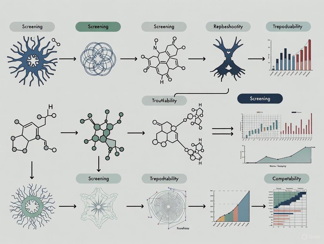
Conceptual Workflow Diagram
The following diagram illustrates the logical relationship between the key concepts of reproducibility, replicability, and robustness, and how they build toward generalisable knowledge.
The Scientist's Toolkit: Essential Research Reagent Solutions
This table details key materials and tools essential for ensuring reproducibility in experimental research, particularly in fields like biochemical screening.
Table: Essential Reagents and Tools for Reproducible Research
| Item | Function in Ensuring Reproducibility | Key Considerations |
|---|---|---|
| Authenticated Cell Lines | The foundational biological reagent for in vitro assays. Using misidentified or contaminated lines invalidates all subsequent results. | Regularly authenticate using STR profiling. Document source, passage number, and culture conditions. Treat cells as validated reagents, not just tools [7]. |
| Assay Guidance Manual (AGM) | A free, comprehensive eBook of best practices for developing robust and reproducible assays for drug discovery. | Provides disease-agnostic standards for assay design, validation, and implementation for HTS and structure-activity relationship (SAR) studies [7]. |
| Version-Controlled Code | Tracks all changes to computational analysis scripts, allowing anyone to recreate the exact analysis at any point in time. | Use systems like Git. Combine with containerization (e.g., Docker) to capture the full software environment. |
| Sample Management System | Ensures sample integrity (e.g., compounds, proteins) by tracking source, concentration, storage conditions, and freeze-thaw cycles. | A strong collaborative relationship between screening and sample handling groups is critical to identify the root cause of assay failure [7]. |
| Statistical Reproducibility Tools | Pre-registration of study design and analysis plans prevents p-value hacking and other forms of unconscious bias [2]. | Clearly define the choice of statistical tests, model parameters, and threshold values before conducting the analysis. |
Troubleshooting Guides
TR-FRET Assay Troubleshooting
Issue: No assay window.
- Cause & Solution: Incorrect instrument setup is the most common reason. Consult your instrument manufacturer's setup guides to ensure compatibility with TR-FRET assays and verify that the correct emission filters are installed. Unlike other fluorescence assays, TR-FRET is exceptionally sensitive to emission filter selection [9].
Issue: Inconsistent EC50/IC50 values between labs.
- Cause & Solution: Differences often originate from variations in compound stock solution preparation. Standardize the preparation of 1 mM stock solutions across all teams and laboratories [9].
Issue: High variability between sample replicates.
- Cause & Solution: Pipetting errors or reagent lot-to-lot variability. Use ratiometric data analysis (acceptor signal/donor signal) to account for small variances in reagent delivery and lot-to-lot differences. Always use a master mix for working solutions [9].
Luciferase Reporter Assay Troubleshooting
Issue: Weak or no signal.
- Cause & Solution: Non-functional reagents, low transfection efficiency, or a weak promoter. Check reagent functionality and plasmid DNA quality. Optimize transfection by testing different DNA-to-transfection reagent ratios. The sample signal must be above the background and negative control [10].
Issue: High background signal.
- Cause & Solution: Contamination or suboptimal plate selection. Use newly prepared reagents and fresh samples. For luminescence assays, use white plates with clear bottoms to reduce background [10].
Issue: High variability between experiments.
- Cause & Solution: Pipetting errors or using different reagent batches. Prepare a master mix, use a calibrated multichannel pipette, and employ a dual-luciferase assay system to normalize data with an internal control reporter [10].
Issue: Signal interference.
- Cause & Solution: Test compounds may inhibit the luciferase enzyme. Avoid known inhibitors like resveratrol, use proper controls, or lower the concentration of the interfering compound [10].
Biochemical Assay General Troubleshooting
Issue: Apparent IC50 value differs from published data.
- Cause & Solution: A 2-3 fold variation is typically within an expected range. Significant differences can arise from variations in assay sensitivity, enzyme-to-substrate ratio, reaction time, or whether a pre-incubation step with the enzyme was used. Adhere strictly to the published protocol and note that values from different assay formats (e.g., colorimetric vs. Mass Spec) are not directly comparable [11].
Issue: Colored compounds interfere with colorimetric readouts.
- Cause & Solution: The compound's intrinsic color absorbs light at the detection wavelength. For each concentration of the colored compound, prepare a separate blank and normalize the assay signal against it [11].
Frequently Asked Questions (FAQs)
Q: What is the difference between IC50 and EC50?
- A: The IC50 (Inhibitory Concentration 50) is the concentration of a compound required to inhibit a biological or enzymatic process by 50%. It is used for inhibitors. The EC50 (Effective Concentration 50) is the concentration required to produce 50% of a maximum desired effect and is used for agonists [11].
Q: How should I design a dose-response experiment to determine an accurate IC50?
- A: Use a serial dilution of your compound in 3-fold increments across 9-10 concentrations. The concentration range must be sufficient to capture the full curve, with the lowest concentrations showing no effect and the highest concentrations showing maximum effect, defining the upper and lower asymptotes of the graph [11].
Q: Can I use cell lysates with my biochemical assay kit?
- A: It is generally not recommended. Biochemical assay kits are designed with validated, recombinant purified proteins to directly test compound effects on a specific target. Using complex cell lysates introduces many uncontrolled variables, making it impossible to confirm the signal's specificity [11].
Q: My assay has a large window but is still not robust. Why?
- A: Assay window alone is an insufficient measure of robustness. Use the Z'-factor, a statistical parameter that incorporates both the assay window size and the variability (standard deviation) of your data. An assay with a Z'-factor > 0.5 is considered excellent for screening. A large window with high noise can have a worse Z'-factor than a small, tight window [9].
Q: What is a homogeneous assay?
- A: A homogeneous assay requires no wash steps to remove unbound molecules, as unbound material does not interfere with the detection signal. This makes it simpler and more amenable to high-throughput screening (e.g., TR-FRET, AlphaScreen). A heterogeneous assay, like an ELISA, requires multiple wash steps [11].
Experimental Protocols
Protocol 1: TR-FRET Ratiometric Data Analysis
Ratiometric analysis is critical for minimizing pipetting and reagent variability in TR-FRET assays [9].
- Collect Raw Data: Obtain Relative Fluorescence Unit (RFU) values for both the donor and acceptor emission channels.
- Calculate Emission Ratio: For each well, divide the acceptor RFU by the donor RFU.
- For a Terbium (Tb) donor: Ratio = RFU (520 nm) / RFU (495 nm)
- For a Europium (Eu) donor: Ratio = RFU (665 nm) / RFU (615 nm)
- Normalize Data (Optional but Recommended): To express data as a normalized response ratio, divide all emission ratio values by the average emission ratio of the negative control (bottom of the curve). This sets the assay window starting at 1.0 and does not affect the IC50 calculation [9].
- Plot and Analyze: Graph the normalized ratio against the logarithm of the compound concentration to generate your dose-response curve.
Protocol 2: Determining IC50 for an Enzyme Inhibitor
This protocol outlines the steps for a biochemical enzyme inhibition assay [11].
- Compound Preparation:
- Dissolve the compound in 100% DMSO at a high concentration (e.g., 10-100 mM).
- Perform a serial dilution in DMSO using 3-fold increments to create a 10-point dilution series.
- Further dilute the compound in assay buffer, ensuring the final concentration of DMSO is constant (e.g., 0.1-1%) across all wells, including controls.
- Assay Setup:
- In a low-binding 96-well plate, combine the diluted compound, enzyme, and substrate in assay buffer according to the kit protocol.
- Include critical controls: a "no compound" control (100% enzyme activity), a "no enzyme" control (background signal), and if available, a control with a known inhibitor.
- Reaction and Detection:
- Incubate the plate under the recommended conditions (time, temperature).
- Develop the assay and read the signal using a compatible plate reader (e.g., fluorescence, luminescence).
- Data Analysis:
- Calculate the percentage of inhibition for each compound concentration:
% Inhibition = [1 - (Signal_compound - Signal_background) / (Signal_no_compound - Signal_background)] * 100 - Plot the % Inhibition vs. the Log10 of the compound concentration.
- Fit the data using a four-parameter logistic (4PL) curve fit to determine the IC50 value.
- Calculate the percentage of inhibition for each compound concentration:
Data Presentation
Table 1: Quantitative Metrics for Assay Validation and Reproducibility
| Metric | Formula / Description | Interpretation | Reference | ||
|---|---|---|---|---|---|
| Z'-factor | `1 - [3*(σpositive + σnegative) / | μpositive - μnegative | ]` | > 0.5: Excellent assay for screening. | [9] |
| Assay Window | (Signal at top of curve) / (Signal at bottom of curve) | A fold-change; however, a large window does not guarantee a good Z'-factor. | [9] | ||
| IC50 | Concentration causing 50% inhibition. | A measure of compound potency; lower value = greater potency. | [11] | ||
| EC50 | Concentration causing 50% of max effect. | A measure of agonist effectiveness; lower value = greater potency. | [11] |
Table 2: Research Reagent Solutions for Enhanced Reproducibility
| Reagent / Tool | Function in Assay | Impact on Reproducibility |
|---|---|---|
| Automation-ready Consumables (e.g., SpecPlate) | Meniscus-free, defined optical pathlength plates for UV/Vis. | Eliminates dilution steps and pipetting errors; ideal for HTS automation [12]. |
| Biomimetic Barrier Systems (e.g., PermeaPad) | Synthetic barrier for passive permeability studies. | Provides a consistent, animal-free model that is more reproducible than variable cell-based systems [12]. |
| Fluorescent Ligands (for HCS) | Non-radioactive probes for studying ligand-receptor interactions in live cells. | Enables real-time, high-content kinetic readouts with improved safety and subcellular resolution [13]. |
| Master Mixes | A single, homogeneous mixture of all assay reagents. | Reduces pipetting variation and well-to-well variability, standardizing reaction conditions [9] [10]. |
| Validated Reference Inhibitors/Agonists | Internal controls provided with or purchased for assay kits. | Serves as a benchmark for assay performance and cross-experiment comparison [11]. |
Workflow and Signaling Pathway Diagrams
Assay Troubleshooting Flow
HCS vs Traditional Assay Workflow
Reproducibility is a fundamental challenge in biochemical screening assays, with over 50% of preclinical results estimated to be irreproducible, costing billions annually in research funds [14]. For researchers and drug development professionals, identifying and controlling the root causes of variability is essential for generating reliable, decision-grade data. This guide addresses three major sources of variability—reagent stability, environmental factors, and protocol deviations—providing actionable troubleshooting and FAQs to enhance the rigor of your experimental workflows.
Troubleshooting FAQs
1. My assay shows high background. What should I check? High background is frequently caused by insufficient washing, which fails to remove unbound components [15]. Ensure you are following the recommended washing procedure precisely. You can increase the number of washes or add a 30-second soak step between washes to improve stringency. Also, verify that you are using fresh plate sealers and reservoirs for each step, as reused materials can harbor residual HRP enzyme that causes high background [15].
2. I have achieved a standard curve, but my sample readings are inconsistent (poor duplicates). What are the likely causes? Poor duplicates typically point to issues with liquid handling or plate condition [15]. First, check your washing process; if using an automatic plate washer, ensure all ports are clean and unobstructed. Second, assess your pipetting technique and ensure all reagents are at room temperature before use to minimize volumetric errors. Finally, uneven plate coating or a poor-quality plate that binds unevenly can also cause this issue [15].
3. My assay results are inconsistent from one run to the next (poor assay-to-assay reproducibility). How can I fix this? This often stems from uncontrolled variables between runs [15]. Key areas to standardize include:
- Protocol Adherence: Strictly follow the same protocol from run to run, avoiding any modifications.
- Incubation Conditions: Adhere to the recommended incubation temperature and times. Avoid incubating plates in areas with environmental fluctuations [15].
- Reagent Preparation: Check calculations and prepare fresh standard curves and buffers for each run. Using internal controls can also help normalize data across runs [15].
4. I suspect a new lot of reagent is causing a shift in my results. What is the best way to investigate this? Perform a reagent lot crossover study [16]. Run a set of patient samples or quality controls using both the old and new reagent lots in the same assay. Compare the results to determine if the difference is statistically and clinically significant. CLSI guidelines provide detailed frameworks for designing these studies [16]. If an unacceptable bias is found, you may need to request a replacement lot from the manufacturer or, after appropriate validation, apply a correction factor [16].
5. What environmental factors are most critical to control in a testing laboratory? Several environmental factors must be monitored and controlled to ensure assay accuracy [17]:
- Temperature: Critical for reagent stability, enzyme kinetics, and proper operation of volumetric equipment.
- Humidity: High humidity can cause hygroscopic materials to absorb moisture, altering their weight and composition.
- Vibrations: Can disrupt sensitive equipment like analytical balances and cause settling or stratification in samples.
- Air Quality: Airborne particles and chemical vapors can contaminate samples or reagents.
Troubleshooting Guide: Common Problems and Solutions
Table 1: Common ELISA Issues and Solutions
| Problem | Possible Source | Recommended Test or Action |
|---|---|---|
| High Background | Insufficient washing [15] | Increase wash number; add 30-second soak step [15]. |
| Contaminated buffers or reused plate sealers [15] | Use fresh plate sealers and reservoirs; make fresh buffers. | |
| No Signal | Incorrectly prepared or old reagents [15] | Check calculations; make new buffers/standards; use new standard vial. |
| Reagents added in wrong order [15] | Review and repeat protocol, ensuring correct order. | |
| Poor Duplicates | Uneven coating or poor plate quality [15] | Use a qualified ELISA plate; check coating volumes and method. |
| Pipetting error [15] | Ensure reagents are at room temperature; check pipette calibration. | |
| Poor Assay-to-Assay Reproducibility | Variations in incubation temperature/time [15] | Adhere strictly to recommended protocols; avoid areas with temperature fluctuations. |
| Buffer contamination or improper standard prep [15] | Make fresh buffers and standard curves for each run. | |
| Edge Effects | Uneven temperature across plate [15] | Use plate sealers; avoid incubating plates on uneven surfaces. |
Table 2: Environmental Factors Impacting Assay Performance
| Factor | Potential Impact on Assays | Control and Monitoring Method |
|---|---|---|
| Temperature | Alters reaction kinetics, reagent stability, and equipment performance [17]. | Use calibrated thermometers; record ambient and incubation temperatures [17]. |
| Humidity | Can cause condensation, alter sample concentration, or impact hygroscopic materials [17]. | Use dehumidifiers/humidifiers; record relative humidity levels [17]. |
| Vibrations | Causes noise in sensitive data and can disrupt equipment alignment [17]. | Use anti-vibration platforms; monitor equipment repeatability [17]. |
| Air Quality | Particulates or chemical vapors can contaminate samples and reagents [17]. | Maintain proper ventilation; use closed containers; track QC sample results [17]. |
| Electrical Supply | Surges or dips can damage instruments or cause reading errors [17]. | Use uninterruptible power supplies (UPS) and voltage stabilizers [17]. |
Experimental Protocols for Validation
Protocol 1: Reagent Stability Testing
Purpose: To determine the in-use and shelf-life stability of critical reagents, ensuring consistent performance over time.
Method (Isochronous Design) [18]:
- Aliquot and Storage: On Day 0, prepare multiple identical aliquots of the reagent and store them under the recommended conditions (e.g., -20°C).
- Scheduled Removal: On each scheduled test day (e.g., Day 1, 7, 30, etc.), remove one aliquot from storage and immediately transfer it to a presumed stable storage condition (e.g., -70°C or lower) to halt further degradation.
- Final Batch Testing: At the end of the study period, test all aliquots—including a freshly prepared one (Day 0 control)—in a single, randomized batch experiment. This minimizes inter-assay variability.
- Data Analysis: Compare the performance of each time-point aliquot against the Day 0 control. The stability limit is the longest duration for which the reagent's performance (e.g., measured signal, recovery of a known concentration) remains within pre-defined acceptance criteria (e.g., ±5% deviation) [18].
Protocol 2: Plate Uniformity Assessment
Purpose: To validate the performance and signal variability of an assay across the entire microplate before commencing high-throughput screening [19].
Method (Interleaved-Signal Format) [19]:
- Plate Layout: Create a plate layout that interleaves "Max," "Min," and "Mid" signal controls across the plate. For example, in a 96-well plate, assign wells for maximum signal (H), minimum signal (L), and a mid-point signal (M) in a patterned fashion (e.g., Figure 1 below).
- Assay Execution: Run the assay according to your protocol over multiple days (e.g., 3 days for a new assay) using independently prepared reagents each day.
- Data Analysis: Calculate the Z'-factor for each day to assess the assay's robustness and signal window. Analyze the data for spatial patterns (e.g., edge effects, row/column biases) that indicate environmental non-uniformity.
- Z'-factor: A statistical measure of assay quality. A Z'-factor > 0.5 is generally considered excellent for screening.
Protocol 3: Reagent Lot Crossover Study
Purpose: To evaluate the equivalence of a new reagent lot against the current lot before implementation.
Method [16]:
- Sample Selection: Select a panel of 5-10 patient samples or quality control materials that span the assay's reportable range (low, mid, and high concentrations).
- Testing: Assay all selected samples with both the current (old) reagent lot and the new reagent lot in the same run, preferably in duplicate or triplicate.
- Statistical Analysis: Perform linear regression and Bland-Altman analysis to compare results. The laboratory must pre-define acceptance criteria for bias (e.g., mean difference < 5%) based on the medical requirements of the test [16].
The Scientist's Toolkit: Key Research Reagent Solutions
Table 3: Essential Materials for Managing Reagent Variability
| Item | Function | Best Practice Guidance |
|---|---|---|
| ELISA Plate (Qualified) | Solid phase for antibody binding. | Use plates designed for ELISA, not tissue culture [15]. |
| Reference Standards & Controls | Calibrate the assay and monitor performance. | Handle according to directions; use new vials for critical assays [15]. |
| Stable, Low-Background Substrate | Generates detectable signal (e.g., color, light). | Mix and use immediately; protect from light [15]. |
| Liquid Handling Equipment (Calibrated) | Accurate and precise dispensing of reagents. | Calibrate regularly; use correct pipettes and tips; ensure tips are sealed [14]. |
| Plate Sealer (Disposable) | Prevents evaporation and contamination during incubation. | Use a fresh sealer for each assay step; do not reuse [15]. |
| Documented Stability Data | Provides manufacturer's data on reagent shelf-life. | Follow storage and in-use stability claims; conduct in-house verification [18]. |
Assay Validation and Troubleshooting Workflows
Assay Troubleshooting Logic Flow
Reagent Lot Validation Decision Flow
Frequently Asked Questions (FAQs)
Q1: A recent survey suggested that over 70% of researchers have been unable to reproduce other scientists' experiments, and over 50% have been unable to reproduce their own. What are the primary factors contributing to this reproducibility crisis? [20] [21]
A1: The reproducibility crisis in life science research, including single-cell transcriptomics, stems from several interconnected factors [20] [21]:
- Lack of access to data and materials: Reproducibility is hindered when raw data, protocols, and key research materials like authenticated cell lines are not readily shared [20].
- Poor experimental design and research practices: Studies designed without a thorough review of existing evidence or with insufficient blinding and randomization are less likely to be reproducible [20].
- Inability to manage complex datasets: Many researchers lack the tools or training to properly analyze, interpret, and store the large, complex datasets generated by modern technologies like single-cell RNA sequencing (scRNA-seq) [20] [22].
- Cognitive and reporting biases: Confirmation bias and the under-reporting of negative or null results skew the scientific literature, making it difficult to assess the true state of knowledge [20].
- Competitive academic culture: The pressure to publish novel, positive findings in high-impact journals often de-incentivizes the careful, repetitive work required for reproducibility [20].
Q2: In single-cell RNA-seq analysis, my cluster results seem to change every time I re-run my analysis with slightly different parameters. How can I stabilize my findings?
A2: Cluster instability is a well-known source of irreproducibility in single-cell genomics [23]. It is common for reanalysis of the same dataset to find 20% fewer or more clusters, with only 50-70% equivalence in cell-type assignments [23]. This arises from numerous analytical decisions. To improve robustness:
- Transparent Reporting: Clearly document all criteria and parameters used for quality control, normalization, highly variable gene selection, and the clustering algorithm itself [23].
- Internal Reproducibility Evaluation: Assess the robustness of your clusters by performing permutations. For example, randomly remove 10% of cells and re-cluster the remainder; a meaningful fraction of cells will often reassign to a different cluster. Reporting a reproducibility metric, like a Rand Index, from such an exercise is recommended [23].
- Define Core Clusters: Consider designating only the cells that consistently cluster together across permutations as a "core" population for downstream analysis, while treating cells with ambiguous identity separately [23].
Q3: My single-cell experiment has data from thousands of individual cells. Can I treat these individual cells as biological replicates for statistical testing when comparing conditions?
A3: No, this is a critical mistake that leads to a high false-positive rate. Treating cells as independent replicates is a statistical error known as sacrificial pseudoreplication, as it confounds variation within a sample with variation between samples [24]. Cells from the same biological sample are correlated. One study found that analyses ignoring sample variation had false positive rates between 30-80%, while methods accounting for it had rates of 2-3% [24].
- Correct Approach: Pseudobulking. A standard correction is to use a "pseudobulk" approach. This involves summing or averaging read counts for each cell type within each biological sample first. Traditional bulk RNA-seq differential expression methods (e.g., DESeq2, limma) are then applied to these sample-level summaries [24].
Q4: I am planning my first single-cell RNA-seq experiment. What are the most common pitfalls during sample preparation, and how can I avoid them?
A4: Success in scRNA-seq starts long before sequencing. Common pitfalls and their solutions include [25]:
- Inappropriate Cell Suspension Buffer: The presence of media, DEPC, RNases, magnesium, calcium, or EDTA can interfere with the reverse transcription reaction. Solution: Wash and resuspend cells in EDTA-, Mg2+-, and Ca2+-free 1x PBS or a recommended FACS collection buffer [25].
- Delayed Processing: RNA degradation begins immediately after cell collection. Solution: Process samples immediately after plating or snap-freeze them in dry ice and store at –80°C until processing [25].
- Low Viability and High Debris: Low viability can lead to sequencing mostly ambient RNA instead of cellular transcriptomes. Solution: Aim for cell preparations with >90% viability and minimal debris [24].
- Skipping Pilot Experiments: Different cell types have varying RNA content. Solution: Always run a pilot experiment with a few samples and controls to optimize parameters like PCR cycle numbers for your specific cell type [25].
Troubleshooting Guides
Issue 1: High Background in Negative Controls
- Potential Cause: Contamination from the environment, amplicons from previous PCR reactions, or reagents.
- Solution: Practice stringent RNA-seq lab techniques. This includes wearing a clean lab coat and gloves, changing gloves frequently, and maintaining physically separated pre- and post-PCR workspaces. Using a clean room with positive air flow for pre-PCR work greatly decreases contamination risk [25].
Issue 2: Low cDNA Yield After Reverse Transcription
- Potential Cause 1: The reverse transcription reaction is being inhibited by components in your sample buffer.
- Potential Cause 2: The starting RNA mass is too low or the protocol is not optimized for your cell type.
- Solution: Perform a pilot experiment. Use a positive control with a known amount of RNA (e.g., 10 pg for single cells) to confirm your technique. Adjust the number of PCR cycles based on the expected RNA content of your cells [25].
Issue 3: Inconsistent Clustering Results
- Potential Cause: The inherent variability and numerous decision points in the scRNA-seq analytical pipeline.
- Solution: Adopt a standardized workflow for internal validation [23].
- Documentation: Meticulously record all parameters for QC, normalization, and clustering.
- Permutation Test: Systematically remove a random subset (e.g., 10%) of cells or samples and re-run your clustering pipeline.
- Calculate a Reproducibility Metric: Use a metric like the Rand Index to quantify the agreement between original and new cluster assignments.
- Refine Clusters: Use the results to define a stable set of "core" clusters for robust downstream analysis.
Quantitative Data on Reproducibility
The following tables summarize key quantitative findings from studies on research reproducibility.
Table 1: Survey Data on Reproducibility Challenges
| Finding | Field | Source | Reference |
|---|---|---|---|
| Over 70% of researchers could not reproduce another scientist's experiments. | Biology | Nature Survey (2016) | [20] |
| Over 50% of researchers could not reproduce their own experiments. | Biology | Nature Survey (2016) | [20] [21] |
| Only 20-25% of validation studies were "completely in line" with original oncology reports. | Oncology Drug Development | Prinz et al. | [26] |
| Only 6 out of 53 "landmark" preclinical studies could be confirmed. | Oncology | Begley & Ellis | [26] |
| An estimated $28 billion per year is spent on non-reproducible preclinical research. | Preclinical Research | Meta-analysis (2015) | [20] |
Table 2: Single-Cell RNA-seq Sample Preparation Guidelines
| Parameter | Recommendation | Purpose | Source |
|---|---|---|---|
| Cell Concentration | 1,000 - 1,600 cells/µL | Optimal for cell capture in droplet-based systems (e.g., 10X Genomics). | [24] |
| Total Cell Number | 100,000 - 150,000 cells | Ensures sufficient material for loading and recovery of target cells. | [24] |
| Viability | >90% | Reduces sequencing of background RNA from dead/dying cells. | [24] |
| Buffer | Mg2+/Ca2+-free PBS, 0.04% BSA | Prevents inhibition of the reverse transcription reaction. | [25] [24] |
Experimental Protocols & Workflows
Detailed Protocol: Preparing a Single-Cell Suspension for 10X Genomics
Principle: To isolate a suspension of live, single cells free of contaminants that inhibit downstream enzymatic reactions [25] [24].
Materials:
- Tissue sample or cell culture
- Appropriate dissociation reagents (e.g., collagenase, trypsin)
- EDTA-, Mg2+- and Ca2+-free 1x Phosphate-Buffered Saline (PBS)
- Bovine Serum Albumin (BSA)
- Cell strainer (e.g., 40 µm)
- Trypan Blue or other viability dye
- Automated cell counter or hemocytometer
Procedure:
- Dissociation: Dissociate tissue using a validated mechanical and/or enzymatic protocol (consult resources like the Worthington Tissue Dissociation Database).
- Quenching & Washing: Quench enzymatic activity with a complete medium. Centrifuge the cell suspension and wash the pellet with 1x PBS + 0.04% BSA.
- Filtration & Counting: Pass the cell suspension through a 40 µm cell strainer to remove aggregates. Take an aliquot to count cells and assess viability using Trypan Blue exclusion.
- Resuspension: Centrifuge and resuspend the cell pellet in PBS + 0.04% BSA at the target concentration of 1,000 - 1,600 cells/µL. The total cell count should be >100,000 cells.
- Storage & Transport: Keep the cell suspension on ice and process it as quickly as possible to minimize RNA degradation and transcriptome changes.
Visual Guide: Single-Cell RNA-Seq Wet-Lab to Dry-Lab Workflow
The following diagram outlines the key steps in a single-cell RNA-seq experiment, highlighting critical decision points that impact reproducibility.
Single-Cell RNA-Seq Workflow and Reproducibility Checkpoints
The Scientist's Toolkit: Essential Research Reagent Solutions
Table 3: Key Reagents and Materials for scRNA-seq Experiments
| Item | Function | Critical Consideration |
|---|---|---|
| Authenticated Cell Lines | Source of biological material; ensures genotype and phenotype are as expected. | Using misidentified or cross-contaminated cell lines invalidates results. Use low-passage, authenticated materials [20]. |
| Unique Molecular Identifiers (UMIs) | Short nucleotide barcodes that label individual mRNA transcripts during reverse transcription. | Allows for accurate transcript counting by correcting for PCR amplification bias, crucial for quantitative accuracy [22] [24]. |
| Cell Barcodes | Short nucleotide barcodes that label all mRNA from a single cell. | Enables pooling of thousands of cells in a single reaction while retaining the ability to deconvolute data back to individual cells [24]. |
| RNase Inhibitors | Protects the fragile RNA template from degradation during sample preparation. | Essential for working with low-input RNA to preserve transcriptome integrity [25]. |
| Mg2+/Ca2+-Free Buffer | Suspension medium for cells during sorting and loading. | Prevents chelation of reaction components and inhibition of reverse transcriptase enzyme [25]. |
Core Concepts: Reproducibility and Metrology
What does "reproducibility" mean in the context of biochemical screening?
Reproducibility is a multi-faceted concept. The scientific community often distinguishes between these key types [20] [27]:
- Methods Reproducibility: The ability to repeat the exact same experimental procedures using the same materials, data, and methodologies as the original study. This relies on complete disclosure of protocols, reagents, and analytical code [27].
- Results Reproducibility (Replicability): Obtaining similar results through an independent study that closely matches the procedures of the original work [27].
- Inferential Reproducibility: Drawing qualitatively similar conclusions from a re-analysis of the original data or an independent dataset [27].
What is a "metrology mindset" and why is it critical for assay development?
A metrology mindset is the formal application of the science of measurement to your experimental workflow. It involves understanding that every measurement result is an estimate, and its quality is defined by a rigorous assessment of its measurement uncertainty (MU) [28]. This mindset shifts the goal from simply getting a result to understanding the confidence and reliability of that result, which is the foundation of reproducible science [29].
What is Measurement Uncertainty (MU), and how is it different from error?
Measurement Uncertainty (MU) is a quantitative parameter that characterizes the dispersion of values that can be reasonably attributed to the analyte being measured [28]. Unlike "error," which is the difference from a true value, uncertainty acknowledges that a true value is often unknowable and instead establishes an interval (e.g., Confidence Interval) around your result where the true value is expected to lie with a given probability [28].
Table: Key Differences Between Error and Uncertainty
| Feature | Error | Uncertainty |
|---|---|---|
| Definition | Difference between measured and true value | Estimate of the dispersion of values attributable to the measurand |
| Concept | Theoretical, often unknowable | Practical, can be quantified |
| Systematic Components | Correctable if known | Accounted for in the uncertainty budget even after correction |
| Final Output | A single value | A value with a defined interval (e.g., ± U) |
Troubleshooting Guides: Common Reproducibility Issues
FAQ: My assay lacks a robust signal window (e.g., low Z'-factor). What should I check?
A poor assay window, quantified by a low Z'-factor (a key metric for assay robustness where >0.5 is suitable for screening), often stems from instrumental or reagent issues [9].
Troubleshooting Steps:
- Verify Instrument Setup: For fluorescent assays like TR-FRET, the single most common reason for failure is an incorrect choice of emission filters. Confirm your instrument's filter settings against the assay's requirements [9].
- Check Reagent Integrity: Ensure reagents are stored correctly and have not expired. Test new lots of critical reagents to rule out degradation or manufacturing variability.
- Confirm Protocol Execution: Review pipetting accuracy, incubation times, and temperatures. Small deviations can significantly impact the signal-to-noise ratio. Automated liquid handlers can minimize human error in these steps [30].
FAQ: I cannot reproduce a published IC₅₀ value. Where did I go wrong?
Differences in calculated potency (IC₅₀ or EC₅₀) between labs are frequently traced to foundational preparation steps [9].
Troubleshooting Steps:
- Stock Solution Preparation: This is the primary reason for EC₅₀/IC₅₀ discrepancies. Pay close attention to how compound stock solutions are prepared (e.g., solvent, concentration accuracy) and stored [9].
- Reagent Authentication: Are you using the same biological materials? Using misidentified, cross-contaminated, or over-passaged cell lines is a major contributor to irreproducible results. Always use authenticated, low-passage reference materials and document their source [20].
- Methodological Detail: Published methods may omit critical details like buffer preparation order ("20 mM HEPES pH 7.2, 150 mM NaCl" is not the same as "20 mM HEPES, 150 mM NaCl, pH 7.2") or specific instrument models. Contact the corresponding author for clarification if needed [31].
FAQ: My experimental data is noisy and inconsistent from day to day. How can I stabilize it?
Day-to-day variability points to a lack of procedural control and environmental stability.
Troubleshooting Steps:
- Control for Cognitive Bias: Implement blinding and randomize sample processing orders to prevent subconscious influences like confirmation bias [20].
- Thoroughly Document Methods: Create and adhere to detailed Standard Operating Procedures (SOPs) that report key parameters such as blinding, instrumentation, number of replicates, statistical analysis methods, and criteria for data inclusion/exclusion [20].
- Robust Data Management: Complex datasets require proper tools for analysis, interpretation, and storage. A lack of these tools can lead to inconsistencies in how data is processed between runs [20].
Experimental Protocols for Enhancing Reproducibility
Protocol: Assessing Assay Robustness with Z'-Factor
The Z'-factor is a standard statistical measure for assessing the quality and robustness of high-throughput screening assays [9].
Methodology:
- Run Controls: Perform your assay in a microtiter plate, designating wells for a positive control (e.g., 100% inhibition) and a negative control (e.g., 0% inhibition). Include a sufficient number of replicates for each (e.g., n≥16).
- Calculate Means and Standard Deviations: For both the positive control (PC) and negative control (NC), calculate the mean (μ) and standard deviation (σ) of the signal.
- Apply the Z'-Factor Formula:
Z' = 1 - [ 3*(σ_pc + σ_nc) / |μ_pc - μ_nc| ] - Interpret the Result:
- Z' > 0.5: An excellent assay suitable for screening.
- 0 < Z' ≤ 0.5: A marginal assay that may need optimization.
- Z' < 0: A "yes/no" type assay; there is no separation between the controls.
Table: Z'-Factor Interpretation Guide
| Z'-Factor Value | Assay Quality Assessment | Suitability for HTS |
|---|---|---|
| Z' > 0.5 | Excellent | Excellent |
| 0 < Z' ≤ 0.5 | Marginal / Doable | May require optimization |
| Z' < 0 | Unacceptable | No (overlap between controls) |
Workflow: A Metrology-Based Approach to Assay Development
The following diagram outlines a systematic workflow for developing assays with a metrology mindset, focusing on identifying and controlling for sources of uncertainty.
The Scientist's Toolkit: Essential Research Reagent Solutions
Using high-quality, well-characterized reagents is non-negotiable for reproducible research.
Table: Key Research Reagents and Their Functions in Ensuring Reproducibility
| Item | Function & Importance in Reproducibility | Best Practice |
|---|---|---|
| Authenticated Cell Lines | Embodies the biological system under study. Misidentified or contaminated lines render all data invalid [20]. | Use repositories that provide STR DNA profiling and regular mycoplasma testing [20] [32]. |
| Validated Antibodies | Key reagent for detection in assays like ELISA or Western Blot. Non-specific binding causes false results [31]. | Use application-validated antibodies and report the clone/catalog number. |
| Reference Standards | Provides a known baseline to calibrate instruments and validate assay performance across time and locations [29]. | Use traceable, certified reference materials where available. |
| High-Purity Biochemicals | Components of assay buffers and solutions. Impurities can introduce unexpected inhibition or activation. | Source from reputable suppliers and document lot numbers. |
| Automated Liquid Handlers | Performs repetitive liquid dispensing tasks. Minimizes human error and variability in pipetting, a major source of noise [30]. | Implement for critical reagent addition; ensure regular calibration. |
Uncertainty Budget: A Top-Down Model for Biochemical Assays
Given the complexity of biological systems, a full "bottom-up" uncertainty calculation as described in the Guide to the Expression of Uncertainty in Measurement (GUM) is often impractical [28]. A "top-down" model that uses existing quality control data is recommended.
Methodology:
- Identify Major Sources: List the main factors contributing to variability in your result (e.g., pipetting volume, temperature fluctuation, operator skill, reagent lot).
- Quantify Contributions: Use data from internal quality control (IQC) and method validation studies to assign a standard uncertainty (u) to each major source. For example, the long-term standard deviation of your IQC material can be a key contributor.
- Combine Uncertainties: Calculate the combined standard uncertainty (u_c) using the root sum of squares method:
u_c = √(u₁² + u₂² + u₃² ...). - Calculate Expanded Uncertainty: Multiply the combined standard uncertainty by a coverage factor (k), typically k=2 for a 95% confidence interval, to get the expanded uncertainty (U):
U = k * u_c[28].
This process creates an "uncertainty budget" that tells you which factors are most responsible for variability in your measurements, allowing you to focus optimization efforts where they matter most.
Building a Robust Foundation: Assay Development and Optimization Strategies
Reproducibility is a fundamental requirement in biochemical screening and drug discovery. A lack of it wastes resources, erodes trust in scientific findings, and significantly hampers the development of new therapies [20]. The selection of an appropriate detection platform is a critical decision that directly impacts the reliability and reproducibility of your data. This technical support center provides troubleshooting guides and FAQs for three prevalent technologies: Fluorescence Polarization (FP), Time-Resolved Förster Resonance Energy Transfer (TR-FRET), and Luminescence. The following sections are designed to help you identify, understand, and resolve common issues, ensuring your assays are robust and your results are reproducible.
Detection Platform Fundamentals and Selection Guide
Understanding the core principles of each technology is the first step in selecting the right platform and effectively troubleshooting problems. The table below summarizes the fundamental mechanisms and common applications of FP, TR-FRET, and Luminescence assays.
Table 1: Core Principles of FP, TR-FRET, and Luminescence Assays
| Platform | Detection Principle | Typical Assay Format | Key Advantages |
|---|---|---|---|
| Fluorescence Polarization (FP) | Measures the change in molecular rotation of a fluorescent tracer upon binding [33]. | Binding assays (protein-ligand, protein-DNA), enzymatic assays. | Homogeneous ("mix-and-read"), ratiometric, no separation steps required, real-time kinetics [33]. |
| TR-FRET | Measures energy transfer from a long-lifetime donor (e.g., Tb) to an acceptor when in close proximity [34]. | Protein-protein interactions, kinase activity, target engagement. | Reduced background due to time-gated detection, ratiometric, suitable for complex biological samples [34]. |
| Luminescence (e.g., ADP-Glo) | Measures light output from an enzymatic reaction (e.g., luciferase) proportional to analyte like ADP [35]. | Enzyme activity (kinases, ATPases), cell viability, reporter gene assays. | High sensitivity, large dynamic range, minimal background from compound autofluorescence. |
The following diagram illustrates the core signaling mechanism for each detection technology.
Troubleshooting Common Assay Issues: FAQs
Fluorescence Polarization (FP) Assays
Q: My FP assay has a very small assay window (low signal-to-noise ratio). What could be the cause? A: A small assay window often stems from an inappropriate tracer or issues with the detection system.
- Tracer Size: Ensure the molecular volume difference between the free and bound tracer is large enough. FP is most sensitive for interactions between a small molecule (<1.5 kDa) and a large partner (>10 kDa) [33].
- Fluorophore Choice: Traditional green dyes (e.g., FITC) can be affected by compound autofluorescence. Switching to red-shifted dyes (e.g., Cy3B, Cy5, BODIPY TMR) can minimize this background interference [33].
- Instrumentation: Verify that your microplate reader is properly configured for FP. Monochromators are not recommended due to low light transmission; optical filters are preferred. Also, ensure the instrument uses a xenon lamp for UV range excitation [33].
Q: I am observing high background or inconsistent polarization values. How can I resolve this? A: This can be caused by compound interference or light scattering.
- Compound Interference: Test compounds can be fluorescent themselves (autofluorescence) or can quench the tracer's signal. It is good practice to measure the fluorescence background of wells containing only the compound and buffer, and subtract this value from the final calculation [33].
- Light Scattering: Precipitated compounds or particles in the solution can scatter light, causing artifacts. Centrifuging assay plates before reading or using red-shifted dyes can help mitigate this issue [33].
TR-FRET Assays
Q: My TR-FRET assay has no assay window. What is the most common reason? A: The single most common reason for a failed TR-FRET assay is the use of incorrect emission filters on your microplate reader [9]. Unlike other fluorescence assays, TR-FRET requires specific filter sets to accurately capture the donor and acceptor signals while minimizing cross-talk and background. Always consult your instrument's compatibility guide and use the recommended filters for your specific TR-FRET reagent.
Q: The TR-FRET signal is weak, even with the correct filters. What should I check? A: A weak signal can be due to several factors related to reagent quality and assay conditions.
- Reagent Quality: Antibodies and other protein reagents can exhibit lot-to-lot variance (LTLV). Impurities like aggregates or fragments can lead to high background and reduced specific signal [36]. Always use authenticated, high-quality reagents and test new lots before full implementation.
- Donor-Acceptor Pair: Ensure spectral overlap is optimal. The donor's emission must efficiently excite the acceptor. For example, a Terbium (Tb) donor has characteristic emissions that should overlap with the acceptor's absorption spectrum [34].
- Assay Components: Confirm that all components, including tags, antibodies, and buffers, are compatible and at optimal concentrations.
Luminescence Assays
Q: My luminescence-based kinase assay (e.g., ADP-Glo) shows high variability and false positives/negatives. Why? A: Luminescence assays can be susceptible to compounds that interfere with the luciferase enzyme itself.
- Luciferase Inhibitors: Some compounds directly inhibit the firefly luciferase used in the detection step, leading to a false decrease in signal that can be mistaken for inhibition [35]. This was demonstrated in a screen where Gentian violet was a false positive in a scintillation assay but was correctly identified as a luminescence inhibitor [35].
- Troubleshooting Step: Implement a counterscreen or a confirmatory assay using a different detection technology (e.g., a radiometric method like SPA) to triage hits and eliminate these format-specific false positives [35].
Q: The luminescence signal is low across all wells, including controls. A: This typically indicates a problem with the assay reagents or protocol.
- Reagent Stability: Luciferase reagents can be unstable. Ensure reagents are fresh, have been stored properly, and are protected from light. Thaw and prepare them according to the manufacturer's protocol.
- ATP Contamination: In assays measuring ADP, trace amounts of ATP in buffers or from enzyme preparations can cause high background. Use ultrapure water and high-quality reagents.
- Protocol Timing: Luminescence signals can decay over time. Ensure a consistent and appropriate incubation time between reagent addition and reading on the plate reader.
Essential Research Reagent Solutions
The quality and consistency of core reagents are paramount for assay reproducibility. The following table outlines key materials and their functions, with a focus on mitigating lot-to-lot variance.
Table 2: Key Research Reagents and Their Roles in Assay Reproducibility
| Reagent Category | Specific Examples | Critical Function | Considerations for Reproducibility |
|---|---|---|---|
| Fluorescent Tracers | T2-BODIPY-FL, T2-BODIPY-589 [34] | Binds to the target of interest; generates the primary signal in FP/TR-FRET. | Purity, labeling efficiency, and spectral properties must be consistent. Cross-platform tracers can enhance data comparability [34]. |
| Antibodies | Anti-6xHis-Tb (for TR-FRET) [34] | Binds to tagged proteins; serves as a donor in TR-FRET. | Aggregates or fragments can cause high background [36]. Use SEC-HPLC and CE-SDS to monitor purity and stability across lots [36]. |
| Enzymes | Luciferase, Horseradish Peroxidase (HRP) [36] | Generates or modulates the detectable signal in luminescence/colorimetric assays. | Quality is measured in activity units, which can vary between batches. Source enzymes from reputable suppliers with consistent QC. |
| Antigens/Proteins | Recombinant kinases, calibrator peptides [36] | The target or standard for the assay. | Purity, activity, and stability are critical. SDS-PAGE and SEC-HPLC are key for assessing quality. Synthetic peptides should be checked for truncated by-products [36]. |
| Cell Lines | Engineered reporter lines, primary cells | Provides the cellular context for the assay. | Authenticate cell lines regularly (e.g., via STR DNA profiling) to avoid misidentification and cross-contamination, a major source of irreproducible data [20] [32]. |
Experimental Protocol: A Cross-Platform Tracer Evaluation
This protocol outlines how to evaluate a fluorescent tracer for cross-platform utility in both TR-FRET and NanoBRET (a luminescence-based technique), a strategy that can enhance data consistency in drug discovery campaigns [34].
Objective: To determine the performance of a fluorescent tracer (e.g., T2-BODIPY-FL or T2-BODIPY-589) in both TR-FRET and cellular NanoBRET target engagement assays.
Materials:
- Purified, tagged protein of interest (e.g., His-RIPK1)
- Tracer compound (e.g., T2-BODIPY-FL, T2-BODIPY-589)
- Anti-tag TR-FRET antibody (e.g., Anti-6xHis-Tb)
- TR-FRET assay buffer
- Cell line expressing the NanoLuc-fused protein of interest
- NanoBRET substrate (e.g., furimazine)
- Opti-MEM or other suitable assay medium
- White, solid-bottom microplates (e.g., 384-well)
- Multi-mode microplate reader capable of TR-FRET and BRET detection
Method: Part A: TR-FRET Assay Optimization
- Prepare Reagents: Dilute the His-tagged protein, anti-6xHis-Tb antibody, and tracer in TR-FRET assay buffer to their working concentrations.
- Titration: In a 384-well plate, serially dilute the tracer across a range of concentrations (e.g., 0.1 nM to 10 µM).
- Reaction Assembly: For each well, mix the protein, antibody, and diluted tracer. Include controls without protein (for background) and without tracer (for donor-only signal).
- Incubation: Incubate the plate in the dark at room temperature for 1-2 hours to reach equilibrium.
- Signal Detection: Read the plate on a TR-FRET-compatible microplate reader. Test different filter pairs (e.g., 520/490 nm, 640/490 nm) to find the optimal signal-to-background ratio for your tracer [34].
- Data Analysis: Calculate the TR-FRET ratio (Acceptor Emission / Donor Emission). Plot the ratio against the tracer concentration to determine the equilibrium dissociation constant (Kd) and the Z'-factor to assess assay robustness [34].
Part B: NanoBRET Assay Evaluation
- Cell Preparation: Seed the NanoLuc-fused protein-expressing cells into a 384-well plate and culture until they reach the desired confluence.
- Tracer Treatment: Dilute the tracer in assay medium and add it to the cells. Include a control with a high concentration of an unlabeled inhibitor to define non-specific binding.
- Substrate Addition: Add the NanoBRET substrate (furimazine) according to the manufacturer's instructions.
- Signal Detection: Incubate briefly and read the plate on a luminescence-compatible reader capable of dual-emission detection (e.g., 460 nm and 610 nm LP filter). A monochromator can be used to optimize detection parameters [34].
- Data Analysis: Calculate the BRET ratio (Acceptor Emission / Donor Emission). A specific signal over background indicates successful cellular target engagement. The Z'-factor should be calculated to confirm assay quality [34].
The workflow for this cross-platform evaluation is summarized below.
Universal assay platforms promise a streamlined approach to analyzing multiple biological targets simultaneously, offering significant advantages in throughput, cost, and sample conservation. However, realizing this potential requires careful navigation of platform-specific challenges to ensure reliable and reproducible results. This technical support center is designed within the broader context of troubleshooting reproducibility issues in biochemical screening assays. It provides researchers, scientists, and drug development professionals with targeted FAQs and evidence-based guides to diagnose, understand, and resolve common experimental problems, transforming complex data into credible biological insights.
Understanding Reproducibility in Universal Assays
Reproducibility—the precision of measurements under varying conditions like different locations, operators, or measuring systems—is a fundamental challenge in assay development [37]. From a measurement science (metrology) perspective, confidence in research results is built not just on reproducibility, but on a systematic understanding of all sources of measurement uncertainty [37].
Universal platforms consolidate multiple experimental steps, but this integration can also combine and amplify sources of variability. Key concepts include:
- Reproducibility vs. Repeatability: Repeatability refers to precision under identical, short-term conditions, while reproducibility assesses precision across expected variations in the real world [37].
- Sources of Uncertainty: These can be diverse, including incomplete definition of the measurand, non-representative sampling, inadequate knowledge of environmental effects, and personal bias [37].
Frequently Asked Questions & Troubleshooting Guides
1. We observed high inter-assay variability in our multiplex immunoassay. What could be the cause?
High inter-assay variability, or poor reproducibility, often points to systematic issues in the assay platform or its execution.
- Possible Causes and Solutions:
- Plate-to-Plate Variability: Irregularities in the manufacturing process, such as inconsistent spotting of capture antibodies, can cause significant variability between lots or even plates from the same lot [38].
- Action: Request lot-validation data from the supplier and consider implementing a pre-rinse step with a PBS/Tween-20 solution to mitigate spotting irregularities [38].
- Insufficient Washing: Inadequate washing can lead to high background signal and poor precision [15].
- Action: Increase the number of wash steps, add a 30-second soak step between washes, and ensure automated plate washer ports are clean and unobstructed [15].
- Sample Matrix Effects: Components in patient samples (e.g., lipids, debris) can interfere with detection [39].
- Action: Clarify samples by centrifugation (5-10 minutes) and ensure at least a 1:1 ratio of sample to assay diluent. For cell lysates, dilute to reduce detergent concentration to ≤0.01% [39].
- Plate-to-Plate Variability: Irregularities in the manufacturing process, such as inconsistent spotting of capture antibodies, can cause significant variability between lots or even plates from the same lot [38].
2. Our high-throughput screen yielded an unusually high number of active compounds. How can we identify false positives?
A high hit rate often signals interference from the compound library itself rather than true biological activity.
Common Types of Compound Interference [40]:
- Compound Aggregation: Molecules form colloids that non-specifically sequester proteins.
- Compound Fluorescence: Chemicals fluoresce at wavelengths used for detection.
- Luciferase Inhibition: Compounds directly inhibit the firefly luciferase reporter enzyme.
- Redox Reactivity: Compounds interfere with the assay's redox potential.
Strategies for Mitigation:
- Include Detergent: Adding 0.01–0.1% non-ionic detergent (e.g., Triton X-100) to the assay buffer can disrupt compound aggregates [40].
- Employ Orthogonal Assays: Confirm hits using a secondary assay with a different detection technology or reporter (e.g., switching from luminescence to fluorescence) [40].
- Utilize Counter-Screens: Run a parallel assay designed specifically to identify common interferers, such as a standalone luciferase inhibition assay [40].
3. We are getting no signal in our ELISA when one is expected. What should we check?
A lack of signal indicates a failure in the assay's detection system.
- Troubleshooting Steps [15]:
- Verify Reagent Integrity: Ensure the standard has been handled correctly and has not expired. Make new buffers to rule out contamination.
- Check Protocol Adherence: Confirm that all reagents were added in the correct order and that the detection antibody and enzyme conjugate (e.g., streptavidin-HRP) were used at the recommended concentrations.
- Confirm Plate Coating: Use plates designed for ELISA, not tissue culture plates. Ensure the capture antibody was diluted in an appropriate buffer (e.g., PBS) without extraneous protein during the coating step.
- Review Instrument Settings: Check that the plate reader is using the correct wavelengths and is functioning properly.
Troubleshooting Guide at a Glance
The table below summarizes common issues, their potential origins, and recommended actions.
| Problem | Potential Cause | Recommended Action |
|---|---|---|
| High Background [15] | Insufficient washing | Increase wash steps; add a soak step; check plate washer. |
| Poor Duplicates [15] | Uneven coating or washing | Use fresh plate sealers; ensure consistent pipetting and reagent addition. |
| Poor Assay-to-Assay Reproducibility [38] [15] | Plate-to-plate variability; protocol drift | Adhere strictly to protocol; use internal controls; validate new reagent lots. |
| Low or No Signal [15] | Degraded reagents; incorrect procedure | Make fresh buffers/standards; check calculations; review protocol steps. |
| Apparent High Activity in HTS [40] | Compound interference (e.g., aggregation) | Add detergent to buffer; perform orthogonal/counter-screens. |
Experimental Protocols for Validation & Troubleshooting
Protocol 1: Validating a Multiplex Immunoassay Platform
This protocol is based on a systematic evaluation of the Searchlight platform and can be adapted for validating any multiplex assay [38].
- Objective: To assess the accuracy, intra-assay, and inter-assay reproducibility of a multiplex platform prior to use in a large clinical study.
- Materials:
- Multiplex assay kit (e.g., Human 9-plex cytokine array).
- Corresponding singleplex assay kits (e.g., from R&D Systems) for comparison.
- Recombinant protein standards.
- Pooled normal human plasma and relevant patient samples (e.g., EDTA plasma from critically ill patients).
- Plate washer and appropriate imaging or detection instrument.
- Methodology:
- Spike and Recovery: Spike recombinant proteins into normal plasma at concentrations within the standard curve range. Assay in triplicate on both the multiplex and singleplex platforms. Calculate percent recovery.
- Intra-Assay Variability: Measure identical patient samples in replicate on the same plate on the same day. Calculate the coefficient of variation (CV%).
- Inter-Assay Variability: Measure identical patient samples on different days using different plates from the same lot. Calculate the CV% for this comparison.
- Platform Comparison: Assay identical patient samples on both the multiplex and singleplex platforms to compare absolute values and correlation.
- Data Analysis: A well-validated platform should demonstrate efficient spike recovery (>70-80%) and low intra- and inter-assay CVs (e.g., <15%). High inter-assay CVs suggest significant plate-to-plate variability [38].
Protocol 2: Confirming Target Engagement in HTS
This protocol outlines steps to triage hits from a high-throughput screen to eliminate false positives [40].
- Objective: To distinguish genuine bioactive compounds from those causing assay interference.
- Materials:
- Hit compounds from primary HTS.
- Reagents for orthogonal and counter-screen assays.
- Non-ionic detergent (e.g., Triton X-100).
- Methodology:
- Retest in Primary Assay: Confirm initial activity.
- Test for Detergent Sensitivity: Re-test hits in the primary assay buffer supplemented with 0.01% Triton X-100. A significant loss of activity suggests the hit may be an aggregate [40].
- Orthogonal Assay: Test all confirmed hits in an assay that measures the same biology but uses a fundamentally different detection method (e.g., a cell-based functional assay vs. a biochemical binding assay).
- Counter-Screen: Test hits in an assay designed to detect the specific interference mechanism suspected (e.g., a luciferase inhibitor counter-screen for a luminescence-based primary assay).
- Data Analysis: Genuine hits will typically maintain activity in the orthogonal assay and show no activity in specific counter-screens. Compounds whose activity is abolished by detergent or that are active in counter-screens are likely false positives.
The Scientist's Toolkit: Essential Research Reagents
The table below lists key materials and their functions for ensuring robust and reproducible assay performance.
| Item | Function | Example & Notes |
|---|---|---|
| Control Probes & Slides [41] | Verifies sample RNA quality and assay performance. | RNAscope control slides (e.g., Human HeLa Cell Pellet); PPIB/UBC (positive), dapB (negative). |
| Universal Assay Buffer [39] | Provides a consistent matrix for diluting samples and standards. | Thermo Fisher Universal Assay Buffer (Cat. No. EPX-11110-000). Reduces matrix effects. |
| Non-Ionic Detergent [40] | Disrupts compound aggregates in HTS, reducing false positives. | Triton X-100, used at 0.01-0.1% in assay buffer. |
| Internal Controls [15] [42] | Monitors assay performance and reproducibility across runs. | Technopath Multichem IA Plus QC materials; in-house pooled controls with known analyte levels. |
| Plate Sealers [15] | Prevents evaporation and contamination; reused sealers can cause contamination. | Use a fresh, non-reusable sealer for each incubation step. |
| ELISA Plates [15] | Optimized surface for antibody binding. | Use plates designed for ELISA, not tissue culture plates, for efficient capture antibody binding. |
Pathways & Workflows
Troubleshooting Pathway for HTS Hit Validation
This workflow provides a logical sequence for confirming that active compounds from a screen are genuine hits.
Multiplex Immunoassay Validation Workflow
A systematic approach to validating a new multiplex platform before committing precious clinical samples.
Reproducibility forms the cornerstone of scientific advancement, yet biomedical research faces a significant challenge, often termed a "reproducibility crisis." Evidence from metastudies suggests only between 10% to 40% of published research is reproducible [27]. A 2016 survey of 1,576 researchers revealed that over 70% have tried and failed to reproduce another scientist's experiments, and more than 50% could not replicate their own findings [21] [14] [20]. This widespread issue erodes trust, wastes resources—estimated at $28 billion annually in the U.S. alone on non-reproducible preclinical research—and slows scientific progress [21] [14] [27].
A critical, often-overlooked factor contributing to this problem is the inadequate qualification and stability testing of research reagents. Variability in reagent performance, driven by improper storage, handling, or a simple lack of understanding of their stability profile, introduces a hidden variable that can invalidate experimental results. This technical support center is designed to provide researchers, scientists, and drug development professionals with targeted troubleshooting guides and FAQs, framed within a broader thesis on troubleshooting reproducibility issues. Our focus is on establishing systematic protocols for reagent qualification, stability testing, and storage optimization to ensure data integrity and experimental robustness.
Understanding Reproducibility: Definitions and Core Concepts
To effectively troubleshoot, it is essential to define key terms often used interchangeably. Based on guidelines from the Association for Computing Machinery and other scholarly efforts, we adopt the following definitions [27]:
- Repeatability: Obtaining consistent measurement results with stated precision by the same team using the same measurement procedure, system, and operating conditions in the same location on multiple trials.
- Replicability: A different group of researchers yields consistent results with stated precision using the same measurement procedure and system, under the same operating conditions, in the same or a different location.
- Reproducibility: An independent group obtains consistent results using a different measuring system, in a different location on multiple trials.
Furthermore, Goodman et al. (2016) refine the concept of research reproducibility into three dimensions [27]:
- Methods Reproducibility: The ability to obtain sufficient detail about study procedures and data to repeat the exact same workflows.
- Results Reproducibility: The ability to obtain consistent results through an independent study closely matching the procedures of the original one.
- Inferential Reproducibility: The ability to draw qualitatively similar conclusions from an independent study or a re-analysis of the original research.
Systematic reagent qualification directly addresses the first two dimensions, ensuring that the foundational components of an experiment are consistent, reliable, and fully documented.
Troubleshooting Guides and FAQs
FAQ: Common Reagent and Assay Challenges
Q1: Our laboratory frequently obtains different EC50/IC50 values for the same compound in the same cell-based assay. What are the most likely sources of this variability?
- A: Differences in stock solution preparation are a primary culprit [9]. Ensure consistent solvent use, accurate concentration verification, and proper storage conditions for stock solutions. Furthermore, in cell-based assays, consider whether the compound is being pumped out of the cells or is targeting an inactive form of the protein (e.g., a kinase) when the assay requires the active form [9].
Q2: Why does our TR-FRET assay show no assay window, or why is the signal weaker than expected?
- A: For TR-FRET assays, the single most common reason for failure is the use of incorrect emission filters [9]. Unlike other fluorescence assays, TR-FRET requires specific filter sets recommended for your instrument. First, verify your microplate reader's TR-FRET setup using control reagents. Other causes include improper instrument calibration, reagent degradation, or pipetting inaccuracies [9].
Q3: Our manual ELISA data shows high well-to-well variability and poor reproducibility between technicians. How can we improve this?
- A: Manual ELISA is highly prone to pipetting errors and cross-contamination [14]. Ensure correct pipetting technique, including using the correct pipette and tips, ensuring tips are firmly seated, avoiding air bubbles, and changing tips between every standard, sample, and reagent [14]. Furthermore, do not mix components from different kit lots, pipette in duplicate to identify errors, and do not modify the test procedure, incubation times, or temperatures [14].
Q4: We are using a commercially available antibody, but our immunohistochemistry (IHC) or Western blot results are inconsistent. What should we check?
- A: The reliability of commercially available antibodies is a well-documented contributor to the reproducibility crisis [21]. First, confirm the antibody has been properly validated for your specific application and species. Always include the recommended positive and negative controls. For IHC and ISH assays, a critical step is antigen retrieval optimization, which depends on tissue type, fixation method, and fixation time [43]. Follow manufacturer guidelines precisely and qualify your samples with controls before running target experiments.
Troubleshooting Guide: Microplate Reader Assay Optimization
Microplate readers are complex instruments, and suboptimal settings are a common source of assay variability. The table below summarizes key parameters to troubleshoot.
Table: Troubleshooting Guide for Microplate Reader Assays
| Parameter | Problem | Solution | Best Practice / Impact |
|---|---|---|---|
| Gain Setting | Signal is saturated (too high) or indistinguishable from background (too low). | Adjust gain: use high gain for dim signals, low gain for bright signals [44] [45]. | Use the instrument's auto-gain or Enhanced Dynamic Range (EDR) feature if available to automatically prevent saturation [44] [45]. |
| Focal Height | Signal intensity is lower than expected. | Adjust the distance between the detector and the microplate [44] [45]. | For adherent cells, set focus at the bottom of the well. Ensure consistent sample volumes across the plate [44]. |
| Number of Flashes | High variability between replicate wells. | Increase the number of flashes per measurement to average out noise [44] [45]. | A higher number reduces variability but increases read time. A balance is required; 10–50 flashes are often sufficient [44]. |
| Well-Scanning | Uneven distribution of cells or precipitate causes distorted readings from a single point measurement. | Use orbital or spiral scanning to average signals across a larger area of the well [44] [45]. | Essential for assays with adherent cells or any heterogeneous sample distribution [44]. |
| Microplate Selection | High background noise or weak signal. | Match the microplate to the detection mode: clear for absorbance, black for fluorescence, white for luminescence [44] [45]. | Black microplates reduce background in fluorescence; white microplates reflect and amplify weak luminescence signals [44]. |
| Meniscus Formation | Inaccurate absorbance path length. | Use hydrophobic plates, avoid detergents (e.g., Triton X), or use a path length correction tool if available [44]. | A meniscus distorts the light path, leading to incorrect concentration calculations [44]. |
Systematic Stability Testing: Protocols and Data Presentation
Stability Study Classifications and ICH Guidelines
Stability testing provides evidence on how the quality of a drug substance or reagent varies over time under the influence of environmental factors. The International Council for Harmonisation (ICH) provides standardized guidelines for stability testing. The following table outlines the primary types of stability studies conducted in drug development.
Table: Types of Stability Studies in Drug Development [46]
| Study Type | Storage Conditions | Purpose | Key Application |
|---|---|---|---|
| Long Term | 25°C ± 2°C / 60% RH ± 5% or 30°C ± 2°C / 65% RH ± 5% [46] | To establish the shelf life and recommended storage conditions [46]. | Primary stability study for determining expiration dates. |
| Intermediate | 30°C ± 2°C / 65% RH ± 5% [46] | To moderately increase the degradation rate for a product intended for long-term storage at 25°C [46]. | Provides a bridge when long-term data is unavailable. |
| Accelerated | Elevated temperatures (e.g., 40°C ± 2°C / 75% RH ± 5%) [46] | To increase the rate of chemical degradation or physical change using exaggerated storage conditions [46]. | Predicts stability profile and supports proposed shelf life. |
| In-Use | Simulated "in-use" conditions (e.g., after opening vial) | To establish the period during which a multi-dose product can be used while retaining quality after its container is opened [46]. | Critical for multi-use reagents and drug products. |
Experimental Protocol: Forced Degradation and Stability-Indicating Method Development
This protocol outlines the development of a stability-indicating method for a protein-based reagent, such as insulin, using infrared (IR) spectroscopy to monitor structural integrity [47].
Aim: To develop a method capable of monitoring degradation of a protein reagent under various stress conditions.
Materials:
- Protein reagent (e.g., Insulin formulations)
- Stress condition incubators (e.g., 0°C, 20°C, 37°C, 40°C)
- IR Spectrometer with Attenuated Total Reflection (ATR) accessory
- Centrifugal concentrators (e.g., 3 kDa cutoff)
- Pipettes and sterile tips
Methodology:
- Sample Preparation: Purify protein from formulation excipients using ultrafiltration (e.g., 3 kDa centrifugal concentrators) to achieve ~90% recovery [47].
- Stress Conditions: Aliquot the purified protein and formulated product into sterile tubes. Store aliquots at different temperatures (e.g., 0°C, 20°C, and 37°C) in climatic exposure test cabinets for extended periods (e.g., up to 3 months) [47].
- Weekly Sampling and IR-ATR Measurement:
- Data Analysis:
- Band-Shift Analysis: Monitor the position of the Amide I band (~1650 cm⁻¹), which is sensitive to protein secondary structure (α-helix, β-sheet). A shift in wavenumber indicates structural change [47].
- Spectral Deconvolution: Analyze the second derivative of the spectra in the Amide I region to quantify the percentage of different secondary structures [47].
- Principal Component Analysis (PCA): Use multivariate analysis to classify samples and identify spectral differences due to degradation [47].
This method offers a fast, reliable way to quantify secondary structural changes that correlate with a decrease in bioactivity, providing a more informative quality control tool than traditional HPLC-UV [47].
Quantitative Data from Stability Studies
The following table summarizes exemplary quantitative data from a systematic stability study on insulin, demonstrating how structural integrity can be monitored over time.
Table: Insulin Stability Monitoring via IR-ATR Spectroscopy Amide I Band Position [47]
| Insulin Type | Initial Amide I Peak (cm⁻¹) | Amide I Peak after 1 Month at 37°C (cm⁻¹) | Amide I Peak after 3 Months at 37°C (cm⁻¹) | Interpretation |
|---|---|---|---|---|
| Insulin Detemir (Levemir) | 1651.34 ± 0.29 | 1650.95 [example] | 1650.50 [example] | A downward shift suggests an increase in β-sheet content, potentially indicating aggregation and fibril formation [47]. |
| Insulin Lispro (Humalog) | 1654.00 ± 0.25 | 1653.80 [example] | 1653.45 [example] | A smaller shift may indicate higher stability under stress compared to other analogs. |
| NPH Insulin Human (Protaphane) | 1652.50 [example] | 1651.90 [example] | 1651.20 [example] | A significant shift suggests sensitivity to elevated temperature, requiring strict cold-chain storage. |
Note: Data is illustrative, combining actual published initial measurements with extrapolated examples for educational purposes. Actual data should be generated empirically [47].
The Scientist's Toolkit: Essential Research Reagent Solutions
The following table details key materials and instruments crucial for implementing rigorous reagent qualification and stability testing protocols.
Table: Key Research Reagent Solutions for Qualification and Stability Testing
| Item / Category | Function & Importance in Qualification | Specific Examples / Notes |
|---|---|---|
| Authenticated Biomaterials | Using traceable, low-passage, and genotypically/phenotypically verified cell lines and microorganisms prevents invalidation of data due to misidentification or contamination [20]. | Obtain from reputable biorepositories; routinely test for mycoplasma and authenticate cell lines. |
| Stability Chambers | Provide controlled environments (temperature, humidity) for systematic long-term, intermediate, and accelerated stability studies [46] [47]. | Climatic exposure test cabinets capable of maintaining specific conditions (e.g., 0°C, 20°C, 37°C, 40°C/75% RH) [47]. |
| Analytical Instrumentation | Used for monitoring Critical Quality Attributes (CQAs) like concentration, purity, and structural integrity. | IR-ATR Spectrometer: For protein secondary structure [47]. HPLC-UV/MS: For purity and identity. Microplate Readers: For functional activity assays. |
| Positive & Negative Control Probes | Essential for qualifying sample quality and assay performance in techniques like IHC and ISH. Helps distinguish between assay failure and true negative results [43]. | For RNAscope: PPIB/POLR2A (positive), dapB (negative) [43]. For IHC: relevant tissue controls with known expression. |
| Ultrafiltration Devices | Allow for purification of the active protein from formulation excipients, enabling direct analysis of the molecule's stability [47]. | 3 kDa cutoff centrifugal concentrators. |
| Standardized Buffers & Reagents | Ensure consistency between experiments and lots. Prevents variability introduced by differences in pH, salt concentration, or contaminant ions. | Use high-purity reagents; specify buffer composition precisely (e.g., "20 mM HEPES pH 7.2, 150 mM NaCl" vs. "20 mM HEPES, 150 mM NaCl, pH 7.2") [21]. |
FAQs on Core Optimization Parameters
1. Why is buffer composition so critical for assay reproducibility? The choice of buffer directly influences protein stability, solubility, and activity. Various buffer additives can significantly impact a protein's overall thermal stability, and an unsuitable buffer can lead to protein aggregation at ambient temperatures, causing irregular assay results and poor reproducibility [48]. Incompatibilities between buffer components and detection dyes (e.g., detergents increasing background fluorescence in DSF experiments) are also common sources of failure [48].
2. How does pH specifically affect my enzyme assay? pH controls the ionization state of catalytic residues in the enzyme and the substrate, directly governing enzyme activity. Even small deviations can alter kinetics and lead to inter-laboratory variability. For instance, a study on papain-based dissociation media found that the addition of the cofactor L-cysteine could acidify the solution to pH 6.6, which was cytotoxic to primary neurons. Titrating the pH back to a physiological ~7.4 completely restored cell viability, underscoring pH's profound impact on biological outcomes [49].
3. What is the most efficient strategy for titrating cofactors and substrates? Using a one-factor-at-a-time (OFAT) approach can be slow, taking over 12 weeks for full optimization. A more efficient strategy is the Design of Experiments (DoE) methodology, which uses fractional factorial approaches and response surface methodology to identify significant factors and optimal assay conditions in less than three days. This provides a more detailed evaluation of variable interactions and speeds up the assay optimization process considerably [50].
4. What are the key metrics for validating an optimized assay? A robust, reproducible assay suitable for high-throughput screening (HTS) should be validated with key performance metrics [51]:
- Z'-factor: A statistical parameter assessing the assay's robustness and suitability for HTS. A Z' > 0.5 is typically required.
- Signal-to-Background Ratio: The difference between the positive and negative signals.
- Coefficient of Variation (CV): A measure of the assay's precision and data variability.
Troubleshooting Guides
Problem: Low or No Signal in Activity Assay
| Potential Cause | Investigation | Solution |
|---|---|---|
| Suboptimal pH | Measure the pH of the final reaction mix with a calibrated micro-pH probe. | Titrate pH using a buffering system appropriate for your desired range (e.g., HEPES for ~7.4). Validate spectrophotometrically with phenol red [49]. |
| Missing or Depleted Cofactor | Review literature for essential cofactors (e.g., metal ions). Check reagent certificates of analysis. | Systematically titrate the cofactor concentration in the presence of a fixed enzyme and substrate concentration to determine the optimal level [50]. |
| Incorrect Buffer | The buffer may contain incompatible additives or wrong ionic strength. | Screen different buffers. Avoid detergents or viscous additives if they interfere with your detection method (e.g., fluorescence) [48]. |
Problem: High Background Signal or Poor Reproducibility
| Potential Cause | Investigation | Solution |
|---|---|---|
| Non-specific Cofactor Effects | Run a no-enzyme control with high cofactor concentrations. | Titrate the cofactor to the minimum required concentration, as high levels can promote non-specific binding or reactions [50]. |
| Buffer Contamination | Perform a buffer-only control assay. | Use high-purity reagents and prepare fresh buffer solutions. Ensure automated liquid handlers are calibrated to prevent cross-contamination [30]. |
| Uncontrolled pH Shift | Monitor pH before and after the reaction. | Increase buffer capacity by increasing concentration, or switch to a buffer with a pKa closer to your desired assay pH. |
Quantitative Data for Optimization
Table 1: Phenol Red Absorbance Properties for pH Monitoring
Phenol red is a low-cost, label-free colorimetric pH indicator useful for real-time monitoring in low-volume assays. Its protonation-dependent spectral shifts allow for quantitative pH calculation [49].
| Parameter | Value / Description | Application in Assay Optimization |
|---|---|---|
| Useful pH Range | 6.8 - 8.2 | Ideal for physiological pH conditions. |
| Absorbance Peak (Acidic) | ~430 nm | Dominant peak indicates acidic environment (pH < 7). |
| Absorbance Peak (Basic) | ~560 nm | Dominant peak indicates alkaline environment (pH > 7). |
| Isosbestic Point | ~480 nm | Absorbance is constant, used for reference. |
| Calculation Ratio | R = A560 / A430 | Concentration-independent assessment of sample pH. |
| pKa Calculation | pHstock - log[(A430-Aacid)/(Abase-A560)] | Enables precise pH determination from absorbance values. |
Table 2: Key Parameters for Systematic Assay Optimization
A summary of critical factors to titrate when developing a robust biochemical assay.
| Parameter | Typical Optimization Method | Key Considerations |
|---|---|---|
| Buffer & pH | Titrate pH in 0.2-0.5 unit increments; screen buffer species. | Use a buffer with pKa ±1.0 of desired pH; check for chemical compatibility. |
| Enzyme Concentration | Titrate to find linear range of product formation over time. | Too high can lead to signal saturation; too low causes poor signal-to-noise. |
| Substrate Concentration | Titrate around the known Km value. | Often used at or below Km for inhibitor studies. |
| Cofactor Concentration | Titrate at fixed enzyme and substrate levels. | Essential for metalloenzymes; can affect stability and specificity. |
| Detection Reagent | Titrate concentration and incubation time. | Ensure compatibility with buffer; optimize for signal-to-background. |
Experimental Protocols
Protocol 1: Spectrophotometric pH Measurement and Adjustment Using Phenol Red
This protocol enables precise, low-volume pH adjustment for enzymatic dissociation media or other sensitive solutions [49].
Key Reagents:
- Solution of interest containing phenol red
- NaOH (e.g., 1 M and 5 M) and HCl (e.g., 1 M) solutions for titration
- Reference buffers (pH 4, 7, 10) for pH meter calibration
Methodology:
- Calibration: Calibrate a low-volume pH meter with standard stock solutions (e.g., pH 4, 7, and 10).
- Sample Preparation: Aliquot 1 mL of your solution (e.g., papain in Hibernate-A medium) into a deep-well plate.
- Initial Measurement: Measure the sample's pH with the calibrated probe.
- Parallel Absorbance Reading: Transfer a 250 µL aliquot to a clear-bottom 96-well plate. Measure the absorbance spectrum from 300-800 nm.
- pH Calculation:
- Calculate the ratio R = A560 / A430.
- For precise calculation, use the modified Henderson-Hasselbalch equation with the absorbance values of the stock solution and titrated samples that fall outside the phenol red indicator range (pH <6.8 and >8.2) to determine the pKa and then the sample pH [49].
- Titration and Validation: Titrate the solution with NaOH or HCl, mixing thoroughly after each addition. Repeat steps 3-5 until the target pH is reached, and cross-validate the spectrophotometric reading with the pH meter.
Protocol 2: Rapid Optimization of Buffer, pH, and Cofactors Using Design of Experiments (DoE)
This strategy uses a fractional factorial design to efficiently identify optimal conditions and significant factor interactions [50].
Key Reagents:
- Purified enzyme
- Substrate(s) and cofactor(s)
- Buffers at different compositions and pH values
- Detection reagents
Methodology:
- Define Objective: Set a clear goal, such as maximizing signal-to-background or initial velocity.
- Select Factors: Choose critical factors to optimize (e.g., buffer pH, Mg2+ concentration, substrate concentration, enzyme concentration).
- Design Experiment: Use statistical software to generate a fractional factorial design, which tests multiple factors simultaneously in a reduced number of experiments.
- Run Experiments: Execute the assay according to the experimental design matrix.
- Analyze Data: Fit the response data (e.g., enzyme activity) to a model to identify significant factors and interaction effects.
- Refine with RSM: Use Response Surface Methodology (RSM) to fine-tune the critical factors identified in the initial screen and locate the precise optimum conditions.
Signaling Pathways & Workflows
The Scientist's Toolkit: Research Reagent Solutions
Table 3: Essential Reagents for Biochemical Assay Optimization
| Reagent / Material | Function in Optimization | Key Considerations |
|---|---|---|
| HEPES Buffer | Provides stable buffering in the physiological pH range (7.2-7.6). | Does not require a CO2 atmosphere, unlike bicarbonate buffers [49]. |
| Phenol Red | Low-cost, label-free colorimetric pH indicator for real-time monitoring. | Absorbance peaks at ~430 nm (acidic) and ~560 nm (basic); useful range 6.8-8.2 [49]. |
| Polarity-Sensitive Dye (e.g., Sypro Orange) | Fluorescent dye used in Differential Scanning Fluorimetry (DSF) to monitor protein thermal unfolding. | Incompatible with detergents and viscous buffer additives that increase background fluorescence [48]. |
| Universal Assay Kits (e.g., Transcreener) | Homogeneous, "mix-and-read" assays that detect universal enzymatic products (e.g., ADP, SAH). | Simplifies development for multiple targets within an enzyme family; adaptable for HTS [51]. |
| Automated Liquid Handler (e.g., I.DOT) | Provides non-contact, precision dispensing of nL volumes. | Enhances reproducibility, enables miniaturization, conserves precious reagents, and reduces human error [30]. |
Implementing Mix-and-Read Homogeneous Assays to Minimize Variability and Simplify Automation
What are the fundamental advantages of mix-and-read homogeneous assays in screening?
Mix-and-read homogeneous assays are designed to eliminate washing and separation steps, enabling all reaction components to be combined and measured in a single well. This "add, mix, and measure" format provides several critical advantages for biochemical screening [52] [53]:
- Reduced Variability: Fewer liquid handling steps minimize opportunities for human error and pipetting inconsistencies.
- Automation Compatibility: Homogeneous formats are inherently suited for high-throughput screening (HTS) automation in 384-well and 1536-well plate formats.
- Simplified Workflows: The elimination of separation steps streamlines protocols and reduces overall assay time.
- Miniaturization Potential: Homogeneous assays work effectively at reduced volumes, conserving precious reagents and samples.
How do homogeneous assays directly address reproducibility challenges in research?
Reproducibility challenges often stem from complex multi-step protocols where cumulative errors compound. Homogeneous assays address this by:
- Minimizing Manipulation: Each transfer or washing step introduces potential variance; homogeneous assays eliminate these entirely.
- Standardizing Protocols: Simplified "mix-and-read" workflows are more easily replicated across different laboratories and operators.
- Enabling Robust Statistical Validation: The simplified workflow contributes to better assay performance metrics, particularly Z'-factor, which is a key indicator of assay robustness and reproducibility [52].
Core Principles and Detection Technologies
What detection methods are commonly used in homogeneous assays?
Homogeneous assays employ various detection technologies that don't require physical separation of bound and unbound components:
| Detection Method | Principle | Best Applications | Key Advantages |
|---|---|---|---|
| Fluorescence Polarization (FP) | Measures change in rotational speed of a fluorescent ligand when bound to a larger protein [52]. | Molecular binding interactions, competitive immunoassays. | No washing steps, highly sensitive to molecular size changes. |
| Time-Resolved FRET (TR-FRET) | Uses energy transfer between fluorophores in close proximity [52]. | Protein-protein interactions, kinase assays, immunoassays. | Reduced autofluorescence, high specificity, ratiometric measurement. |
| Fluorescence Intensity (FI) | Measures direct changes in fluorescence signal intensity [52]. | Enzymatic activity, viability assays. | Simple instrumentation, compatible with most plate readers. |
| Luminescence | Detects light emission from chemical or biological reactions [52]. | Cell viability, reporter gene assays, ATP detection. | High sensitivity, broad dynamic range, low background. |
| Electrochemical | Measures electrical signal from redox reactions on sensor surfaces [54]. | Quantification of proteins, viral vectors in crude samples. | Insensitive to sample turbidity or color, label-free. |
How does the "mix-and-read" concept simplify automation?
The simplified workflow of mix-and-read assays translates directly to more reliable automation:
Troubleshooting Guide: Common Issues and Solutions
Poor Signal-to-Background Ratio
Problem: Inadequate difference between positive and negative controls reduces assay robustness and statistical validity.
| Potential Cause | Diagnostic Experiments | Corrective Actions |
|---|---|---|
| Suboptimal reagent concentrations | Titrate enzyme/substrate concentrations in checkerboard pattern; measure signal and background at each combination. | Identify concentration ratio that maximizes signal while minimizing background; use Z'-factor > 0.5 as validation target [52]. |
| Insufficient reaction time | Perform kinetic measurements to monitor signal development over time. | Extend incubation period until signal plateau is reached; ensure consistent timing across all plates in automated runs. |
| Detection reagent degradation | Test fresh vs. stored detection reagents with known controls. | Prepare fresh detection reagents; implement proper storage conditions (often -20°C protected from light). |
| Instrument settings miscalibrated | Verify gain settings and measurement times using control wells. | Optimize plate reader settings specifically for assay plate type (384-well vs. 1536-well). |
High Well-to-Well Variability
Problem: Excessive coefficient of variation (CV) between replicate wells undermines data reliability.
| Potential Cause | Diagnostic Experiments | Corrective Actions |
|---|---|---|
| Inconsistent liquid dispensing | Measure dispensed volumes gravimetrically; test dye distribution across plate. | Calibrate automated liquid handlers regularly; implement non-contact dispensing (acoustic dispensing preferred for nanoliter volumes) [30] [55]. |
| Incomplete mixing | Add dye tracer and measure uniformity across well after mixing step. | Increase mixing duration or speed; ensure consistent mixing across all plate positions; consider alternative mixing technologies. |
| Edge effects (evaporation) | Compare center vs. edge well performance in same plate. | Use proper plate seals; maintain humidity in incubators; include edge well controls in validation. |
| Cell or reagent settling | Monitor signal consistency over time with repeated measurements. | Ensure homogeneous cell/reagent suspensions before dispensing; implement mixing steps before reading. |
Inadequate Z'-Factor for HTS
Problem: Assay robustness metric (Z'-factor) below 0.5 indicates insufficient window for reliable screening.
| Potential Cause | Diagnostic Experiments | Corrective Actions |
|---|---|---|
| High positive control variance | Calculate individual CVs for positive and negative controls. | Optimize control concentrations to maximize separation; ensure control stability throughout assay duration. |
| Signal dynamic range too small | Measure signal range from minimum to maximum possible values. | Increase assay incubation time; evaluate alternative detection technologies with greater dynamic range. |
| Background signal too high | Measure signal in blank wells containing all components except enzyme/target. | Identify and replace components causing high background; implement quenching technologies if available. |
| Temperature fluctuations | Monitor plate temperature throughout assay timeline. | Ensure consistent temperature control during incubation; pre-warm reagents to assay temperature. |
Assay Interference from Compounds or Reagents
Problem: Test compounds or sample components interfere with detection signal.
| Potential Cause | Diagnostic Experiments | Corrective Actions |
|---|---|---|
| Compound autofluorescence | Measure compound alone at assay concentrations. | Switch to non-fluorescent detection method (luminescence, TR-FRET, or electrochemical) [54]. |
| Compound quenching | Test signal recovery with spike-in controls. | Dilute compound to sub-interfering concentrations; implement reagent addition order that minimizes quenching. |
| Sample matrix effects | Compare standards in buffer vs. sample matrix. | Purify or dilute samples; implement standard addition calibration for quantitative assays. |
| Chemical interference with detection | Test detection system with known activators/inhibitors. | Modify detection chemistry; introduce washing step if absolutely necessary (sacrifices homogeneity). |
Advanced Implementation Strategies
How can universal assay platforms simplify multiple projects?
Universal assays detect common products of enzymatic reactions (e.g., ADP for kinases, SAH for methyltransferases), allowing the same detection system to be applied across multiple targets within an enzyme family [52]:
Implementation Protocol:
- Target Assessment: Confirm that your target produces a universal metabolite (ADP, NADH, SAH, etc.).
- Kit Validation: Validate the universal assay with your specific target using positive and negative controls.
- Condition Optimization: Adapt buffer conditions, substrate concentrations, and detection reagent ratios for your target.
- Cross-Validation: Confirm correlation between universal assay and target-specific readout (if available).
What automation considerations are critical for success?
Key Automation Protocols:
- Fixed Volume Approach: Ideal for repetitive dose curves with consistent plate layouts using predetermined pick lists [55].
- Variable Volume Approach: Suitable for flexible screening campaigns where transfer patterns and volumes vary between runs [55].
- Intermediate Dilution Steps: Essential for achieving accurate final concentrations when working with nanoliter dispensing volumes [55].
Essential Research Reagent Solutions
What key reagents and tools enable successful implementation?
| Reagent/Platform | Function | Application Notes |
|---|---|---|
| Transcreener ADP² Assay | Competitive immunoassay detecting ADP production via fluorescence [52]. | Universal kinase assay; mix-and-read format; compatible with FI, FP, or TR-FRET detection. |
| AptaFluor SAH Assay | TR-FRET-based detection of S-adenosylhomocysteine [52]. | Universal methyltransferase assay; works with diverse methyltransferase targets. |
| Chemical Protein Stability Assay (CPSA) | Label-free target engagement measuring ligand-induced protein stabilization [53]. | Uses cell lysates; mix-and-read; identifies binders outside active site. |
| Amperia His-Tag Quantification Kit | Electrochemical detection of His-tagged proteins in crude samples [54]. | Label-free; insensitive to sample turbidity; premix competition format. |
| I.DOT Liquid Handler | Non-contact dispensing with nanoliter precision [30]. | Enables assay miniaturization; reduces reagent consumption by up to 50%. |
| Echo FlexCart System | Acoustic dispensing for compound screening workflows [55]. | Creates assay-ready plates; fixed and variable protocol options. |
Frequently Asked Questions (FAQs)
How can we transition from an ELISA to a homogeneous mix-and-read format?
Transitioning requires identifying a homogeneous detection method that maintains assay specificity:
- Evaluate Alternative Technologies: TR-FRET or FP-based immunoassays can often replace colorimetric ELISA.
- Develop Premix Format: Combine all reagents in a single addition where possible.
- Validate Correlation: Run parallel assays with traditional ELISA and new homogeneous format to ensure equivalent performance.
- Optimize for Automation: Adapt protocol for 384-well or higher density formats with appropriate liquid handling.
What are the most common pitfalls when implementing homogeneous assays for HTS?
- Insufficient Validation: Rushing to screening before thorough optimization of Z'-factor and CV.
- Ignoring Compound Interference: Failing to test for autofluorescence or quenching with representative compounds.
- Volume Inconsistency: Not accounting for evaporation in miniaturized formats, particularly in edge wells.
- Overlooking Reagent Stability: Assuming detection reagents remain stable throughout entire screening campaign.
How do we validate that our homogeneous assay is ready for HTS?
A comprehensive validation should include:
- Statistical Robustness: Z'-factor > 0.5 in at least three independent experiments [52].
- Precision: CV < 10% across replicate wells within a plate and between plates.
- Signal Stability: Consistent performance over at least 4 hours to accommodate automated screening runs.
- Compound Compatibility: Demonstration that DMSO concentrations (typically 0.1-1%) don't interfere with signal.
Can homogeneous assays be used for difficult targets with low expression?
Yes, but requires special considerations:
- Signal Amplification: Consider coupled enzyme systems or other amplification strategies.
- Background Reduction: Implement time-resolved detection (TR-FRET) to minimize autofluorescence.
- Enhanced Detection Sensitivity: Explore next-generation detection technologies with improved sensitivity.
- Sample Pre-concentration: When possible, concentrate samples while maintaining compatibility with homogeneous format.
How do we handle assay miniaturization without losing performance?
Successful miniaturization requires addressing key challenges:
- Liquid Handling Precision: Implement non-contact dispensing for nanoliter volumes [30].
- Evaporation Control: Use proper plate seals and maintain humidity control.
- Mixing Efficiency: Ensure adequate mixing at reduced volumes through optimization.
- Detection Compatibility: Confirm plate readers can reliably detect signals in miniaturized formats.
A Systematic Diagnostic Toolkit: Identifying and Resolving Common Pitfalls
A significant reproducibility crisis affects life science research, with estimates suggesting more than 75% of published data on potential drug targets cannot be replicated [21]. In High-Throughput Screening (HTS), a key lead generation strategy, a major contributor to this problem is the presence of Pan-Assay Interference Compounds (PAINS) [56] [57]. These compounds appear as promising "hits" not through genuine target modulation, but by subverting assay biochemistry, leading to false positives and costly dead-ends. This technical support center provides actionable troubleshooting guides and FAQs to help researchers identify and triage these problematic compounds early, saving valuable time and resources.
Core Concepts: Understanding Assay Interference
FAQ: What are PAINS and Why Are They Problematic?
Q: What exactly are PAINS? A: Pan-Assay Interference Compounds (PAINS) are classes of compounds defined by common substructural motifs that encode a high probability of producing a positive readout in biochemical assays, regardless of the specific target [56] [58]. They function as reactive chemicals rather than specific drugs, and their activity is often non-progressable, meaning they cannot be optimized into viable drug candidates [56].
Q: How common are they in screening libraries? A: A typical academic screening library may contain between 5% to 12% of PAINS [58]. One screening campaign of over 225,000 compounds initially identified 1,500 hits, but further studies revealed that only 3 were true hits—the rest were interferers [58].
Q: What are the common mechanisms of interference? A: PAINS can disrupt assays through multiple mechanisms [56]:
- Chemical Reactivity: Reacting with biological nucleophiles (e.g., thiols, amines) in assay reagents or the target protein.
- Metal Chelation: Binding metals that may be essential for protein function or present as contaminants, interfering with the assay system.
- Redox Activity: Undergoing redox cycling to generate reactive oxygen species that inhibit proteins.
- Spectroscopic Interference: Absorbing light or fluorescing at wavelengths used for detection, skewing readouts.
- Aggregation: Forming colloidal aggregates that non-specifically sequester proteins.
Key PAINS Classes and Their Mechanisms
Table: Common PAINS Classes and Their Characteristic Interference Mechanisms
| PAINS Class | Representative Substructure | Primary Mechanism of Interference |
|---|---|---|
| Enones | ![Enone structure description] | Michael acceptor, reactive with nucleophiles |
| Rhodanines | ![Rhodanine structure description] | Reactive scaffold, redox activity |
| Quinones/Catechols | ![Quinone structure description] | Redox cycling, metal chelation |
| Curcuminoids | ![Curcumin structure description] | Metal chelation, spectroscopic interference |
| Isothiazolones | ![Isothiazolone structure description] | Protein-reactive, electrophile |
| Toxoflavins | ![Toxoflavin structure description] | Redox cycling |
Troubleshooting Guide: Identifying and Confirming Suspect Hits
FAQ: How can I quickly flag potential interferers in my hit list?
Q: What are the first signs that my hit might be a PAINS compound? A: Be suspicious of hits that exhibit one or more of the following characteristics [56] [57]:
- Flat Structure-Activity Relationships (SAR): Potency does not change meaningfully with significant structural modifications.
- Shallow Hill Slopes: In dose-response curves, this can indicate a non-specific mechanism of action.
- Limited Potency Range: A cluster of hits with very similar IC50 values despite diverse structures.
- High Promiscuity: The compound is a known frequent hitter across multiple, unrelated screening campaigns.
Q: Are computational filters reliable for identifying PAINS? A: Electronic PAINS filters are a useful first pass but must be used with caution. They can process thousands of compounds in seconds to flag substructures associated with interference [56]. However, their "black box" use is simplistic and risky [56]. Limitations include:
- They were derived from a specific library and assay technology (AlphaScreen) and are not comprehensive [56].
- A compound not flagged by the filters may still be an interferer [56].
- They may inappropriately exclude a useful compound or tag a useless one as worthy [56]. Always use filters as part of a broader triage strategy.
Experimental Protocol 1: Using a Robustness Set for Assay Validation
A powerful proactive strategy is to test your assay against a "Robustness Set" of known nuisance compounds during development [57].
Objective: To identify and mitigate your assay's inherent vulnerabilities to common interference mechanisms before running a full HTS.
Methodology:
- Assemble the Set: Curate a collection of 50-100 compounds representing various interference classes (e.g., aggregators, redox cyclers, chelators, fluorescent compounds) [57].
- Run the Screen: Screen the robustness set under your primary assay conditions.
- Analyze Hit Rate: Calculate the percentage of robustness set compounds that show activity (e.g., >20% inhibition/activation). An assay inhibited by >25% of the set is considered highly vulnerable and likely to generate excessive false positives [57].
- Refine Conditions: Modify assay conditions to reduce vulnerability. A case study on phosphofructokinase (PFK) showed that adding a reducing agent (2mM DTT) reduced hits from the robustness set from 90% to 9%. Further refinement using a weaker reducing agent (5mM cysteine) virtually eliminated the interference while maintaining assay quality [57].
Experimental Protocol 2: Orthogonal Assays for Hit Confirmation
Objective: To verify that a primary hit engages the target via a specific, desired mechanism.
Methodology: Any primary hit must be confirmed in at least one orthogonal assay with a different detection technology and/or endpoint [57]. The workflow below outlines a rigorous confirmation process.
Key Orthogonal Assays:
- Biophysical Methods:
- Thermal Shift Assay (TSA): Measures protein thermal stability changes upon ligand binding. True binders typically cause a clear shift in the melting temperature, while interferers may produce atypical profiles like shoulders or second peaks [57].
- Surface Plasmon Resonance (SPR): Directly measures binding kinetics in real-time without labels.
- Isothermal Titration Calorimetry (ITC): Measures the heat change from binding, providing information on affinity, stoichiometry, and thermodynamics.
- Counter-Screens:
- Run the hit against an unrelated target using the same assay technology to check for promiscuity.
- Include detergent (e.g., 0.01-0.05% Tween-20) to disrupt aggregate-based inhibition [56].
The Scientist's Toolkit: Essential Reagents and Materials
Table: Key Research Reagent Solutions for PAINS Triage
| Reagent / Material | Function in Triage and Identification |
|---|---|
| Robustness Set Compound Library | A curated collection of known bad actors (aggregators, redox cyclers, etc.) used to validate an assay's vulnerability to interference before full-scale screening [57]. |
| Dithiothreitol (DTT) | A strong reducing agent added to assay buffers (e.g., 2mM) to protect against oxidation-sensitive false positives. Note: can react with some redox cyclers [57]. |
| Tween-20 or Triton X-100 | Detergents added to assay buffers (e.g., 0.01-0.05%) to disrupt and prevent the formation of compound aggregates, a common interference mechanism [56] [57]. |
| Cysteine | A weaker reducing agent (e.g., 5mM) that can mitigate interference from redox-cycling compounds without the reactivity issues sometimes seen with DTT [57]. |
| Chelating Agents (e.g., EDTA) | Used to interrogate metal-dependent interference by chelating free metal ions in the assay buffer. |
| Automated Liquid Handling Systems | Instruments like non-contact dispensers (e.g., I.DOT) improve reproducibility by eliminating cross-contamination and ensuring precise, consistent liquid handling, reducing human error [30]. |
Advanced Triage: Investigating Subtle Interference
FAQ: What about interferers that pass initial checks?
Q: My hit confirms in a secondary assay and isn't flagged by PAINS filters. Could it still be an interferer? A: Yes. Interference can be subtle and context-dependent. Be alert for:
- Metal Contamination: Trace metals from synthesis can co-purify with your compound and cause inhibition. Ciulli et al. reported a case where zinc contamination mediated protein oligomerization, mimicking true inhibition [57].
- "Specific" Aggregators: Some aggregates can form structured assemblies that mimic specific inhibitors. Blevitt et al. described an aggregate of five molecules that mimicked a TNF subunit, causing potent but artifactual inhibition [57].
- Assay-Specific Interference: Some compounds interfere only with specific technologies (e.g., salicylates in FRET assays) and won't be flagged by general PAINS filters [56].
Investigative Protocol: For stubborn, potent hits with unusual properties, advanced techniques like X-ray crystallography can reveal the true mechanism, such as the presence of a mediating metal ion or a specific aggregate structure [57].
Reagent degradation is a fundamental challenge in biochemical screening assays, directly impacting the reproducibility and reliability of research data. Establishing robust stability profiles and accurate expiration times is not merely a regulatory formality but a critical scientific practice to ensure experimental integrity. This technical support center provides actionable guidance and protocols to help researchers systematically address reagent instability, a common source of irreproducibility in biomedicine and drug development.
Foundational Concepts: Stability and Shelf Life
Stability is defined as the extent to which a product retains, within specified limits and throughout its period of storage and use, the same properties and characteristics that it possessed at the time of manufacture [59]. The period during which it remains stable is its shelf life [60].
A product is considered stable as long as its critical characteristics remain within the manufacturer's predefined specifications [60]. For in-vitro diagnostic (IVD) reagents, calibrators, and controls, stability testing ensures performance and functionality throughout the intended shelf life, which is vital for accurate diagnosis and effective patient care [61].
Table 1: Core Stability Testing Terminology
| Term | Definition | Application Context |
|---|---|---|
| Real-Time Stability Testing | Product stored at recommended storage conditions and monitored until failure [60]. | Primary method for definitive shelf-life assignment; required for biologics license applications [61] [59]. |
| Accelerated Stability Testing | Product stored at elevated stress conditions to predict shelf life in a compressed timeframe [60] [61]. | Preliminary claims for new products, supporting modifications to existing products [59]. |
| Shelf Life | The number of days a product remains stable at recommended storage conditions [60]. | Labeled expiration date [61]. |
| In-Use Stability Testing | Evaluates product performance in real-world conditions after opening or reconstitution [61]. | Determining onboard stability on instruments or "after opening" expiry [59]. |
| Expiration Date | The end of the period when a product is expected to meet its specified properties [62]. | Final date of use as determined by real-time or accelerated studies [61]. |
Troubleshooting Guides & FAQs
FAQ: Can I use reagents after their expiration date?
Using expired reagents is a common but risky practice. Manufacturers advise against it, but feasibility depends on several factors. Expired reagents may still be effective if:
- Storage conditions were ideal and matched manufacturer recommendations [62].
- The risk of product degradation is minimal, with a low chance of contamination [62].
- Simple tests are available and used to confirm the reagent's key properties (e.g., pH for a buffer) [62].
However, when the quality of an expired reagent is uncertain, using it poses a significant risk that can compromise experiments and lead to costly irreproducible research [62].
Troubleshooting Guide: Investigating Unexpected Experimental Results
When facing aberrant results, reagent degradation should be a primary suspect. Follow this systematic investigation workflow.
Actions for Key Steps:
- Step 1: Check Reagent Expiry and Storage: Verify the expiration date on the primary container. Confirm that storage temperature, humidity, and light protection have consistently adhered to the manufacturer's label claims [62] [61].
- Step 2: Perform Control Tests: Run the assay with known positive and negative controls. If controls fail to perform as expected, it strongly indicates a problem with the assay reagents or components [59].
- Step 3: Test with Fresh Reagent: Repeat the experiment using a fresh vial of reagent or a newly prepared batch from a different lot, if available. This is the most direct way to isolate the variable.
- Steps 5-7: Quarantine and Investigate: Once a degraded reagent is identified, place all potentially affected product lots on hold. Conduct a failure investigation, including an impact analysis to determine the scope of the problem and affected experiments or batches [59].
FAQ: What is the difference between real-time and accelerated stability testing, and when should I use each?
- Real-Time Stability Tests involve storing a product at its recommended storage conditions and monitoring its performance until it fails the specification. This is the gold-standard method preferred by regulators, but it can take years to complete [60] [61].
- Accelerated Stability Tests subject the product to elevated stress conditions (e.g., higher temperature) to rapidly force degradation. The degradation rate at storage conditions is predicted using known relationships, such as the Arrhenius equation for temperature [60] [59].
Usage Context: Accelerated studies are excellent for preliminary shelf-life claims during development or for validating modifications to an existing product. However, for final product release, especially for biologics, real-time data confirming the accelerated prediction is typically required [61] [59].
Experimental Protocols for Establishing Stability
Protocol 1: Designing a Real-Time Stability Study
This protocol aligns with regulatory expectations for IVDs and can be adapted for research reagents [61] [59].
1. Define Stability Protocol & Acceptance Criteria:
- Before initiation, define a written protocol with predefined acceptance criteria that correlate with the product's label claims and intended use [61] [59]. Criteria should be based on parameters like physical appearance, chemical purity, and functional performance.
2. Select Test Materials:
- Use at least three independent production lots to capture lot-to-lot variation [60] [61].
- Lots should be manufactured under finalized conditions and packaged in the same container-closure system as the marketed product [61].
3. Establish Storage Conditions and Testing Schedule:
- Store materials under the exact conditions stated on the label (e.g., temperature, humidity, light protection) [61].
- Use a statistically valid sample size and testing intervals. Testing should continue for at least one interval beyond the proposed labeled expiration date to fully characterize the degradation trend [61].
4. Employ Validated Test Methods:
- Use reliable, meaningful, and specific test methods to evaluate stability [59]. For reagents, this typically involves performing the functional assay and verifying that results for controls and calibrators meet specifications.
Protocol 2: Executing an Accelerated Stability Study using the Arrhenius Equation
The Arrhenius equation describes the relationship between temperature and the degradation rate, which is fundamental to predicting shelf life [60].
1. Prerequisites and Assumptions:
- The degradation reaction must follow zero- or first-order kinetics at each elevated temperature and at the recommended storage temperature [60].
- The same degradation model must fit the data at each temperature [60].
- The mechanisms of degradation at high temperatures should not differ from those at the recommended storage temperature [60].
2. Experimental Procedure:
- Select Temperature Levels: Choose at least three elevated temperatures that stimulate fast but measurable degradation without destroying the product's fundamental characteristics. Common choices are 4°C, 25°C, 37°C, and 45°C, depending on the reagent's sensitivity [60].
- Conduct Testing: For each elevated temperature, store multiple samples and measure degradation over time. The testing period at elevated temperatures should be sufficient to observe significant degradation.
- Model Degradation: For each temperature, fit the degradation data to a kinetic model (e.g., first-order) to estimate the degradation rate constant (k).
3. Data Analysis and Prediction: The Arrhenius equation is: [ k = A e^{(-E_a/RT)} ] where:
- ( k ) is the degradation rate constant
- ( A ) is the pre-exponential factor
- ( E_a ) is the activation energy
- ( R ) is the universal gas constant
- ( T ) is the temperature in Kelvin
By taking the natural logarithm, the equation becomes linear: [ \ln(k) = \ln(A) - \frac{E_a}{R} \frac{1}{T} ]
- Plot ( \ln(k) ) against ( 1/T ) for the elevated temperatures.
- Fit a linear regression to the data. The slope of the line is ( -E_a/R ).
- Use this regression line to extrapolate and predict the degradation rate (( k_{storage} )) at the recommended storage temperature.
- Calculate the predicted shelf life at storage temperature using the model and the critical degradation level (C) [60].
Table 2: Example Data from a Simulated Accelerated Stability Study
| Temperature (°C) | Estimated Degradation Rate (k) | Time to 80% Activity (Days) |
|---|---|---|
| 35°C | 0.00185 | 217 |
| 30°C | 0.00102 | 392 |
| 25°C (Predicted) | 0.00056 | 714 |
| 4°C (Storage) | Extrapolated from model | Predicted Shelf Life |
Example based on simulated data from [60], assuming first-order kinetics and a critical level of C=0.8 (80% activity).
The Scientist's Toolkit: Key Research Reagent Solutions
Table 3: Essential Materials and Tools for Reagent Stability Management
| Item | Function in Stability Management |
|---|---|
| Authenticated, Low-Passage Cell Lines | Using traceable and authenticated biological reference materials is essential for reliable and reproducible data in cell-based assays [20] [63]. |
| Validated Assays | Assays should be rigorously validated for biological relevance and robustness of performance before being used in stability studies [19]. |
| Electronic Inventory Management System | Platforms (e.g., Quartzy, HappiLabs) track reagent dates, batch numbers, and storage conditions, sending alerts for nearing expirations to prevent waste and use of degraded reagents [62]. |
| Stability Chambers | Provide controlled environments for real-time stability testing, ensuring constant temperature, humidity, and light protection as per label claims [61]. |
| Reference Standards & Controls | Well-characterized materials used in parallel testing to monitor for bias and ensure the consistency and accuracy of stability-testing results over time [59]. |
Proactively establishing stability profiles and expiration dates is a cornerstone of reproducible science. By integrating the troubleshooting guides, experimental protocols, and best practices outlined in this technical support center, researchers and drug development professionals can significantly mitigate the risks associated with reagent degradation. A rigorous, documented approach to reagent management not only safeguards individual experiments but also strengthens the overall credibility and efficiency of the scientific enterprise.
Frequently Asked Questions (FAQs)
Q1: Why is DMSO compatibility testing critical for my biochemical assays? DMSO is not a biologically inert solvent. It can directly interfere with cellular processes and enzymatic activities, leading to false positives, false negatives, and unreliable structure-activity relationship (SAR) data. Testing ensures the biological system tolerates the DMSO concentration used without affecting the assay's outcome [64] [65].
Q2: What is the maximum recommended DMSO concentration for cell-based assays? It is generally recommended to keep the final DMSO concentration under 1% for cell-based assays. However, this is not a universal rule. The acceptable level must be empirically determined for each specific assay system, as some sensitive cell lines show signs of differentiation or toxicity at concentrations as low as 0.125% [19] [66].
Q3: My compound precipitated in DMSO. How does this affect my assay? Compound precipitation in DMSO stock solutions is a major issue. It leads to inaccurate dosing during liquid handling, causing false negatives and an underestimation of compound activity in biological data. Precipitation can occur during initial solubilization or from repeated freeze-thaw cycles [67] [64].
Q4: Can DMSO affect my assay beyond general cytotoxicity? Yes. Recent studies show that DMSO can be metabolized by cells and interfere with specific pathways, particularly sulfur metabolism. It can alter the expression and activity of key enzymes like thiosulfate sulfurtransferase (TST) and cystathionine γ-lyase (CTH), as well as affect glutathione levels, even at non-cytotoxic concentrations [65].
Q5: Why am I getting irreproducible IC50/EC50 values between labs? A primary reason for differing results is variability in the preparation of compound stock solutions. Differences in dissolution, storage conditions (e.g., freeze-thaw cycles), and the resulting compound solubility can lead to significant discrepancies in the final concentrations tested [9].
Troubleshooting Guides
Problem 1: No or Poor Assay Window
An assay window is the signal dynamic range between positive and negative controls. Its absence indicates an inability to detect a compound's effect.
- Potential Causes and Solutions:
- Incorrect Instrument Setup: Confirm that your microplate reader is configured with the exact emission and excitation filters recommended for your detection technology (e.g., TR-FRET) [9].
- Improper Reagent Preparation: Verify that all reagents were reconstituted and stored correctly. Check the stability of critical reagents after freeze-thaw cycles [19].
- Excessive DMSO Concentration: The DMSO solvent itself may be inhibiting the biological reaction. Systematically test the DMSO tolerance of your assay as described in the protocols below [19].
Problem 2: Compound Precipitation
Precipitation is a common issue with high-concentration DMSO stocks and during dilution into aqueous buffers.
- Potential Causes and Solutions:
- Low Intrinsic Solubility: Screen for solubility early. Consider chemical modification of lead compounds to improve solubility or use cosolvents [64].
- Suboptimal Dilution Protocol: Avoid intermediate dilution steps in aqueous buffers. Perform serial dilutions in DMSO and add these directly, in low volumes, to the assay media [64].
- Freeze-Thaw Instability: Store DMSO stock solutions in single-use aliquots to minimize freeze-thaw cycles, which can promote precipitation [67] [64].
Problem 3: Inconsistent Data and High Variability
This refers to high well-to-well or plate-to-plate noise, making it difficult to distinguish true compound effects.
- Potential Causes and Solutions:
- DMSO Evaporation: DMSO is hygroscopic. Ensure sealed storage of stock solutions and use sealed plates during incubation to prevent concentration shifts due to evaporation.
- Edge Effects: Temperature gradients across the microplate can cause uneven DMSO effects. Use proper incubation equipment and consider using plates with sealed edges.
- Liquid Handling Inaccuracy: Precipitated compounds can clog pipette tips. Centrifuge DMSO source plates before use to pellet any precipitate and ensure accurate liquid handling [67].
Experimental Protocols
Protocol 1: DMSO Compatibility Testing
This protocol determines the maximum tolerated DMSO concentration in your assay.
1. Principle: The assay is run in the absence of test compounds but with varying concentrations of DMSO. The concentration that does not statistically alter the control signals ("Max," "Min," "Mid") is selected for screening.
2. Materials:
- Assay buffer and all standard reagents
- 100% DMSO (high-purity, anhydrous)
- Labware compatible with DMSO [68]
3. Procedure: 1. Prepare a dilution series of DMSO in your assay buffer, typically covering a range from 0.1% to 10% [19]. 2. Run your validated assay protocol, replacing the usual buffer with the DMSO/buffer solutions. 3. Include standard "Max," "Min," and "Mid" control signals in each DMSO condition. 4. Perform the experiment over multiple days (e.g., 3 days for a new assay) to assess reproducibility [19].
4. Data Analysis: Calculate the Z'-factor for each DMSO concentration to assess the robustness of the assay window. A Z'-factor > 0.5 is considered excellent for screening [9]. The highest DMSO concentration that maintains a Z'-factor > 0.5 should be selected for production screening.
Table: Example DMSO Compatibility Results for a Hypothetical Enzyme Assay
| Final DMSO Concentration (%) | Max Signal (RFU) | Min Signal (RFU) | Assay Window (Max/Min) | Z'-factor |
|---|---|---|---|---|
| 0.0 | 50,000 | 5,000 | 10.0 | 0.85 |
| 0.5 | 49,500 | 5,100 | 9.7 | 0.82 |
| 1.0 | 48,000 | 5,300 | 9.1 | 0.78 |
| 2.0 | 35,000 | 6,000 | 5.8 | 0.45 |
| 5.0 | 20,000 | 8,000 | 2.5 | 0.15 |
Based on this data, a final DMSO concentration of 1.0% or lower would be appropriate for this assay.
Protocol 2: Assessing Compound Solubility in DMSO Stocks
This protocol evaluates the physical stability of compounds in DMSO.
1. Principle: Visual inspection and light scattering are used to detect particulate matter or precipitation in compound stock solutions over time and after freeze-thaw cycles.
2. Materials:
- Compound stock solutions in 100% DMSO
- Centrifuge for microplates
- Microscope or plate-based nephelometer
3. Procedure: 1. After initial solubilization, visually inspect the stock solution against a dark background. Note any cloudiness or particles. 2. Centrifuge the stock plate (e.g., 1000 × g for 10 minutes) to pellet any precipitate. 3. Quantify precipitation using a nephelometer or by measuring the concentration in the supernatant post-centrifuge and comparing it to the theoretical concentration [67] [64]. 4. Subject aliquots to multiple freeze-thaw cycles (e.g., -20°C to room temperature) and repeat steps 1-3 to assess stability under typical handling conditions.
4. Data Analysis: Compounds with significant precipitation after centrifugation or freeze-thaw cycles should be flagged. For these, consider using fresh stocks for each experiment, using cosolvents, or employing alternative storage methods like dry films [64].
Pathway and Workflow Visualizations
DMSO Interference in Sulfur Metabolism
The diagram below illustrates how DMSO can interfere with cellular sulfur metabolic pathways, a potential source of assay variability.
Experimental Workflow for DMSO/Assay Validation
This workflow outlines the key steps for validating DMSO compatibility and compound integrity in an assay.
The Scientist's Toolkit: Essential Research Reagents and Materials
Table: Key Resources for Managing DMSO and Solvent Effects
| Tool / Reagent | Function & Rationale |
|---|---|
| High-Purity, Anhydrous DMSO | Minimizes water uptake and prevents hydrolysis of test compounds. Ensures consistent starting material for stock solutions [64]. |
| DMSO-Compatible Labware | Use plates and tubes made from materials (e.g., polypropylene) that resist DMSO to prevent leaching of plastics or solvent degradation [68]. |
| Cosolvents (e.g., Ethanol, Acetonitrile) | Alternative or complementary solvents for compounds with very poor DMSO solubility. Note: Each requires its own compatibility testing [68]. |
| Solvent Selection Tool (e.g., ACS GCI Tool) | Interactive tools based on Principal Component Analysis (PCA) of solvent properties to help identify greener or more compatible alternative solvents [69]. |
| Chemical Compatibility Database (e.g., Cole-Parmer) | Reference databases that provide ratings on how different chemicals and solvents interact with various plastics, elastomers, and other materials [70]. |
| Polymerosomes (PEG-PLGA) | An advanced method to encapsulate DMSO, potentially mitigating its direct membrane effects and providing a more controlled delivery system in cell cultures [65]. |
Optimizing Signal-to-Background and Dynamic Range for Robust Detection
Troubleshooting Guides
Weak or No Signal
- Problem: The assay signal is too weak to distinguish from background noise.
- Solutions:
- Reagent Functionality: Check if critical reagents, such as enzymes or detection antibodies, are functional and have not degraded. For bioluminescence assays, ensure substrates like luciferin are freshly prepared and used immediately, as they can lose efficiency over time [71].
- Assay Scale: Scale up the volume of your sample and reagents per well to enhance the signal [71].
- Transfection Efficiency: If using transfected cells, test different ratios of plasmid DNA to transfection reagent to find the optimal efficiency. The signal from samples must be above the background and negative control [71].
- Detection Method: Choose a sensitive detection method, such as fluorescence polarization (FP) or TR-FRET, which provide a broad dynamic range and low background [72].
High Background Signal
- Problem: Excessive background noise obscures the specific assay signal.
- Solutions:
- Microplate Selection: Use black microplates for fluorescence assays to reduce background noise and autofluorescence. For luminescence, use white plates to reflect and amplify weak signals [44].
- Reagent Contamination: Use newly prepared reagents and fresh samples to avoid contamination [71].
- Media Components: For cell-based assays, background noise can be caused by fluorescent molecules in media supplements like Fetal Bovine Serum and phenol red. Consider using microscopy-optimized media or performing measurements in PBS+ [44].
High Variability Between Replicates
- Problem: High coefficient of variation (CV) indicates poor reproducibility between experimental replicates.
- Solutions:
- Pipetting Consistency: Use a calibrated multichannel pipette to minimize pipetting errors. Preparing a master mix for your working solution ensures reagent consistency across wells [71].
- Automated Reagent Dispensing: Use a luminometer with an injector to dispense bioluminescent reagents uniformly [71].
- Data Normalization: Normalize your data using an internal control. In a dual luciferase assay system, the ratio of firefly to Renilla luciferase activity is used to control for variability in cell number and transfection efficiency [71].
- Plate Effects: Identify and mitigate "edge effects" (evaporation in perimeter wells) by using humidity control, plate sealing, or avoiding the use of perimeter wells for critical data [72].
Signal Saturation
- Problem: The signal is too high, exceeding the detector's upper limit and making accurate measurement impossible.
- Solutions:
- Sample Dilution: Perform a serial dilution of your sample lysate to find a concentration that provides a signal within the dynamic range of your detector [71].
- Gain Adjustment: On your microplate reader, lower the gain (signal amplification) setting to prevent detector oversaturation, which results in unusable data [44]. Some advanced readers offer Enhanced Dynamic Range (EDR) technology that automatically adjusts gain during measurements [44].
Signal Instability or Drift
- Problem: The assay signal changes over time during the measurement period.
- Solutions:
- Enzyme Stability: Reagent degradation or enzyme instability can cause drift. Include stabilizers in your buffer or pre-validate storage conditions [72].
- Reaction Linearity: Conduct time-course studies to find an incubation time where product formation is linear and stable. For enzyme assays, aim for only 5–10% substrate conversion during detection to avoid substrate depletion [72].
- Temperature Control: Ensure consistent incubation temperature, as higher temperatures may increase signal but risk enzyme denaturation [72].
Frequently Asked Questions (FAQs)
1. Why is optimizing signal-to-background and dynamic range critical for my screening assay? A robust signal-to-background (S/B) ratio and wide dynamic range are fundamental for reliably distinguishing true hits from inactive compounds in high-throughput screening (HTS). Poor optimization leads to high rates of false positives and false negatives, wasting costly reagents and time [72]. It directly impacts the statistical robustness of your screen and is a key factor in ensuring reproducible results.
2. What is the Z'-factor, and what value should I target? The Z'-factor is a statistical measure of assay quality that incorporates both the dynamic range and the data variation of the positive and negative controls [72].
- Z' > 0.5: Indicates an excellent assay ready for HTS.
- Z' between 0.5 and 0.7: Acceptable for pilot screens.
- Z' < 0.4: Suggests the assay requires further optimization before proceeding [72]. Aim for Z' ≥ 0.6 in 384-well plates whenever possible [72].
3. How can I reduce variability in my luciferase reporter assays? High variability in luciferase assays often stems from pipetting errors, reagent instability, or differences in transfection efficiency. To fix this:
- Prepare a single master mix for your working solution.
- Use a calibrated multichannel pipette.
- Normalize your data using a dual luciferase assay system (e.g., the ratio of firefly to Renilla luciferase activity).
- Use a luminometer with an injector to ensure consistent reagent dispensing [71].
4. Some compounds in my library interfere with the assay signal. How can I address this? Some compounds can inhibit or quench signals from reporter enzymes like luciferase [71]. To manage this risk:
- Avoid known inhibitors if possible.
- Use proper controls, including a detection-only control (without enzyme) to identify signal quenchers or fluorescent artifacts [72].
- Modify incubation time or lower the concentration of the interfering compound [71].
5. My assay has a low Z'-factor. What are the first parameters I should troubleshoot? A low Z'-factor is often caused by a low dynamic range or high variability. Systematically check and optimize these key parameters [72]:
- Reagent Concentrations: Perform a matrix experiment to titrate both the enzyme and substrate concentrations to find the optimal signal response.
- Incubation Time: Ensure the reaction rate is linear over the measurement time.
- Background Noise: Check for autofluorescence from plates or buffer components and switch to low-fluorescence plates if needed.
Key Performance Metrics and Targets
The following table summarizes the key quantitative parameters for a robust assay.
| Parameter | Definition | Optimal Target for HTS |
|---|---|---|
| Z'-Factor | A statistical measure of assay quality and robustness that incorporates the signal dynamic range and the data variation of both positive and negative controls [72]. | ≥ 0.5 (Excellent); Aim for ≥ 0.6 [72] |
| Signal-to-Background (S/B) | The ratio of the signal in the positive control to the signal in the negative control [72]. | As high as possible; specific target depends on assay chemistry. |
| Coefficient of Variation (CV) | The ratio of the standard deviation to the mean, expressing the variability of replicate measurements as a percentage [72]. | < 10% [72] |
| Substrate Turnover | The percentage of substrate converted to product during the detection phase of an enzyme assay [72]. | 5–10% (to maintain linearity and avoid substrate depletion) [72] |
Experimental Protocol: Optimizing a Kinase Assay for Robust Detection
This protocol outlines a systematic approach to optimizing a biochemical kinase assay using a universal detection method, such as ADP detection, to achieve a high Z'-factor and robust signal window [72].
1. Reagent Preparation:
- Purified kinase enzyme.
- Appropriate substrate (e.g., peptide).
- ATP solution.
- Detection reagent (e.g., Transcreener ADP² Assay reagent).
- Reaction buffer.
- Control compounds (known inhibitor for negative control, no-inhibitor for positive control).
2. Enzyme and Substrate Titration (Matrix Experiment):
- Objective: To determine the optimal enzyme and substrate (ATP) concentrations that yield the largest dynamic range and a linear reaction rate.
- Method:
- Titrate the enzyme concentration while keeping the ATP concentration constant.
- In a parallel experiment, titrate the ATP concentration around its known Km value while keeping the enzyme concentration constant.
- Use a multi-well plate to set up the reactions and measure the initial rate of product formation for each condition.
- Plot the signal (e.g., fluorescence intensity) versus concentration for both titrations. The optimal condition is the one that gives the greatest difference between the positive and negative controls (high signal window) with low replicate variability.
3. Reaction Time-Course:
- Objective: To establish the incubation time that ensures linear product formation.
- Method:
- Set up the assay at the optimal enzyme and ATP concentrations identified in Step 2.
- Measure the signal at multiple time points (e.g., 0, 15, 30, 60, 90 minutes).
- Plot the signal versus time. Choose an incubation time that lies within the linear portion of the curve and corresponds to approximately 5-10% substrate conversion [72].
4. Signal Uniformity and Z'-Factor Testing:
- Objective: To validate the assay's robustness across a full microplate.
- Method:
- On a 384-well plate, alternately dispense positive controls (reaction with no inhibitor) and negative controls (reaction with a known inhibitor) across the entire plate.
- Run the assay under the optimized conditions from Steps 2 and 3.
- Calculate the Z'-factor using the formula mentioned in the FAQs. Confirm Z' > 0.7 [72].
- Visualize the data with a plate heatmap to check for any spatial bias (e.g., edge effects).
5. DMSO and Compound Interference Testing:
- Objective: To ensure the assay tolerates the solvent used for compound libraries and is not susceptible to compound interference.
- Method:
- Perform the assay in the presence of a gradient of DMSO (e.g., 0.5%, 1%, 2% v/v) to test for solvent tolerance.
- Include control wells with detection reagent but no enzyme to identify compounds that quench the signal (false negatives) or are auto-fluorescent (false positives) [72].
Experimental Workflow Diagram
The diagram below illustrates the logical workflow for troubleshooting and optimizing your assay.
Troubleshooting Workflow for Assay Optimization
The Scientist's Toolkit: Essential Research Reagents and Materials
The following table details key reagents and materials crucial for developing and optimizing robust biochemical assays.
| Item | Function / Explanation |
|---|---|
| White Microplates | Used for luminescence assays; the white color reflects light, amplifying weak signals [44]. |
| Black Microplates | Used for fluorescence assays; the black plastic reduces background noise and autofluorescence by quenching cross-talk between wells [44]. |
| Hydrophobic Microplates | Minimizes meniscus formation in absorbance and fluorescence assays, which can distort path length and measurements [44]. |
| Universal Detection Reagents | Kits that detect universal nucleotide products (e.g., ADP, GDP). They simplify optimization by allowing a single detection technology to be applied across multiple enzyme targets, reducing variables [72]. |
| Dual Luciferase Assay System | An assay system that sequentially measures firefly and Renilla luciferase activity from the same sample. The ratio of activities is used for data normalization, solving problems with variability in transfection efficiency and cell number [71]. |
| Master Mix | A single, homogenous mixture of all reagents required for a reaction step, distributed across multiple wells. This ensures consistency and minimizes pipetting variability between replicates [71]. |
| Path Length Correction Tool | A feature on some microplate readers that detects the actual path length in each well and normalizes absorbance readings, correcting for meniscus effects or slightly different liquid volumes [44]. |
Frequently Asked Questions (FAQs)
FAQ 1: What does the Hill Coefficient (nH) fundamentally tell me about my experiment?
The Hill coefficient is a quantitative measure of cooperativity in a ligand-receptor or enzyme-substrate interaction [73]. It describes how the binding of one ligand molecule influences the binding of subsequent molecules.
- nH > 1 (Positive Cooperativity): The binding curve is steeper than a hyperbolic one. The binding of the first ligand facilitates the binding of subsequent ligands, making the system more sensitive to small changes in ligand concentration around the EC50/IC50 [73] [74].
- nH = 1 (Non-cooperative Binding): The binding curve is hyperbolic. Ligand binding events are independent of each other, and the system follows Michaelis-Menten kinetics [73].
- nH < 1 (Negative Cooperativity): The binding curve is shallower. The binding of the first ligand hinders the binding of subsequent ligands [73]. In enzymatic dose-inhibition curves, an nH < 1 can indicate that at least one ternary complex retains enzymatic activity [74].
FAQ 2: My Hill coefficient is not an integer. Does this mean my model is wrong?
No, a non-integer Hill coefficient is commonly observed and expected [73] [74]. The original Hill equation was a simplification that considered only the fully occupied macromolecule, ignoring all intermediate complexes [73] [74]. In practice, the Hill coefficient is an empirical measure of the steepness of the dose-response curve and should not be strictly interpreted as the exact number of binding sites, though the maximum possible experimental nH is less than or equal to the number of binding sites involved in the response [74].
FAQ 3: What are the common experimental artifacts that can lead to unreliable Hill coefficients?
Several factors during high-throughput screening (HTS) can compromise data quality and lead to misleading Hill coefficients [75]:
- Systematic Spatial Artifacts: Evaporation gradients, pipetting errors, or temperature drift across assay plates can create patterns (e.g., edge effects, column-wise striping) that distort dose-response relationships [75].
- Compound-Specific Issues: Drug precipitation, chemical instability, or carryover during liquid handling can alter the effective concentration [75].
- Poor Curve Fit: Fitting a 4-parameter logistic (4PL) model to low-quality data with high noise or a weak response can yield nonsensical Hill coefficients (e.g., nH >> 1) that are not justified by the data [74].
FAQ 4: How can I improve the reproducibility of my concentration-response data?
Implementing robust quality control (QC) is essential.
- Go Beyond Traditional Controls: Do not rely solely on control-based metrics like Z-prime. These can miss spatial artifacts in drug wells [75].
- Use Residual Error Analysis: Employ metrics like Normalized Residual Fit Error (NRFE) to identify systematic spatial errors by analyzing deviations between observed and fitted response values across all compound wells. Plates with high NRFE show significantly lower reproducibility among technical replicates [75].
- Automate Liquid Handling: Utilize non-contact, automated dispensers to minimize human error, cross-contamination, and improve precision, especially when working with nanoliter volumes [30].
Troubleshooting Guide
Use the following table to diagnose and address common issues with concentration-response experiments.
| Symptom | Possible Causes | Recommended Solutions & Diagnostic Checks |
|---|---|---|
| Irregular, "jumpy" dose-response curves [75] | • Systematic spatial artifacts on the assay plate (e.g., evaporation, pipetting errors).• Compound precipitation or instability. | • Visualize plate layout to check for column/row patterns.• Calculate the NRFE metric to quantify spatial artifacts [75].• Re-test compound with fresh preparation. |
| Hill coefficient is significantly greater than the number of binding sites | • Poor data quality or fit: The fitted maximum/minimum is outside the error range of controls [74].• Ligand-induced denaturation: The compound causes non-specific protein denaturation [74]. | • Validate fit parameters: Ensure the IC50 is within the tested concentration range and that the fitted max/min are biologically plausible [74].• Compare the fit to a simpler model (e.g., 3-parameter fit). A drastically better fit with the 4-parameter model may not be warranted by the data [74]. |
| Low maximum efficacy and a shallow curve (nH < 1) in an inhibition assay | • The inhibitor is a partial agonist or the ternary complex retains enzymatic activity [74].• Negative cooperativity in binding. | • Confirm mechanism: Use orthogonal assays to verify if the compound is a true antagonist.• Test if a high concentration of the weak partial agonist can block the response of a full agonist to estimate its binding affinity [76]. |
| High variability between technical replicates or studies | • Manual pipetting errors, especially with low volumes [30].• Inconsistent reagent or cell quality.• Undetected spatial artifacts in HTS [75]. | • Automate liquid handling for precision and consistency [30].• Implement rigorous QC: Use a combination of Z-prime (or SSMD) and NRFE to flag and exclude low-quality plates [75].• Ensure proper cell line authentication and reagent standardization [32]. |
Experimental Protocols & Data Interpretation
Standard Protocol for Generating a Dose-Response Curve
This protocol is adapted from common practices in high-throughput screening and biochemical assays [32] [77] [76].
- Plate Preparation: Dispense a wide, log-range of drug concentrations (typically 8-12 concentrations in serial dilution) into assay plates. Include controls for 0% activity (e.g., no enzyme) and 100% activity (e.g., no inhibitor) [77].
- Reaction Initiation: Add a constant concentration of the enzyme/receptor preparation to initiate the reaction. Use automated, non-contact dispensers for reproducibility [30].
- Incubation: Incubate under optimal conditions (temperature, pH) for a predetermined time.
- Signal Measurement: Quantify the response using an appropriate readout (e.g., absorbance, fluorescence, luminescence).
- Data Analysis:
- Normalize the data to the positive and negative controls (0-100% scale).
- Fit the normalized data to the four-parameter logistic (4PL) Hill equation [74] [76]: ( E = E{min} + \frac{(E{max} - E{min})}{1 + 10^{(log(EC{50}) - X) \cdot n{H}}} ) where ( E ) is the effect, ( E{max} ) and ( E{min} ) are the maximum and minimum asymptotes, ( X ) is the logarithm of concentration, ( EC{50} ) is the half-maximal effective concentration, and ( n{H} ) is the Hill coefficient.
- For inhibition assays, the equation is analogous, yielding an ( IC{50} ).
Quality Control Workflow
The following diagram illustrates a robust QC workflow that integrates traditional and novel methods to ensure data reproducibility.
QC Workflow for Reliable Dose-Response Data
Interpreting the Hill Coefficient in Context
The Hill coefficient must be interpreted within the specific biological context.
- Agonist vs. Inhibitor Curves: A dose-response curve for a receptor agonist that requires binding of two ligands to elicit a response (e.g., an ion channel) can show a Hill coefficient > 1, even if the binding to the two sites is independent and non-cooperative. This is because the response is proportional only to the fully occupied receptor complex [74].
- Evidence of Allostery: While a Hill coefficient different from 1 is proof of multiple ligand binding, it cannot by itself distinguish between competitive, non-competitive, or various allosteric mechanisms. Further mechanistic studies are required [74].
Quantitative Data Reference
| Parameter | Symbol | Definition & Interpretation | Typical Range & Notes |
|---|---|---|---|
| Potency | EC50 / IC50 | The concentration that produces 50% of the maximal response (EC50) or 50% inhibition (IC50). A lower value indicates higher potency [77]. | pM to µM. Depends on affinity and system. |
| Efficacy | Emax | The maximal possible response achievable by a drug. Measures the functional strength of an agonist [77]. | 0-100%. For a full agonist, Emax is 100%. |
| Hill Coefficient | nH | Quantifies the steepness of the curve and cooperativity. nH > 1: positive cooperativity; nH < 1: negative cooperativity [73] [74]. | Non-integer values are common. The maximum value is ≤ the number of binding sites [74]. |
| Equilibrium Dissociation Constant | Kd | The ligand concentration at which 50% of receptors are occupied. A measure of binding affinity [73] [77]. | Low Kd = High affinity. May not equal EC50 due to signal amplification. |
The Scientist's Toolkit: Essential Research Reagents & Materials
| Item | Function in Concentration-Response Assays |
|---|---|
| Precision Microplate Readers | Measure absorbance, fluorescence, or luminescence signals from assay plates with high sensitivity and accuracy [74]. |
| Automated Liquid Handlers | Enable precise, high-throughput dispensing of reagents and compounds into microplates, minimizing human error and ensuring consistency [30]. |
| High-Quality Enzyme/Receptor Preparations | Validated identity, mass purity, and enzymatic purity of proteins are critical for generating reliable and reproducible binding or activity data [32]. |
| Stable Cell Lines | Engineered cell lines expressing the target receptor or enzyme are essential for cell-based dose-response assays (e.g., FLIPR assays for GPCR targets) [32]. |
| Standardized Assay Kits | Provide optimized buffers, substrates, and controls for specific target classes (e.g., kinase, protease, GPCR assays), reducing development time and variability [32]. |
Visualizing a Cooperative Binding Mechanism
The following diagram illustrates the classic Monod-Wyman-Changeux (MWC) model for positive cooperativity, which provides a conceptual framework for understanding Hill coefficients > 1.
Allosteric Model of Cooperativity
Ensuring Assay Fitness: From Statistical Validation to Orthogonal Confirmation
FAQs on Core Validation Metrics
What is the Z'-factor and how do I interpret it?
The Z'-factor (Z-prime) is a statistical parameter used to assess the quality and robustness of a screening assay, particularly in high-throughput screening (HTS). It evaluates the assay's signal separation band by comparing the positive and negative control populations [78] [79].
Calculation: Z' = 1 - [3*(σpc + σnc) / |μpc - μnc|] Where σpc and σnc are the standard deviations of the positive and negative controls, and μpc and μnc are their means [79].
Interpretation Guidelines [78] [79] [80]:
- Z' ~ 1: An ideal (but practically unattainable) assay with huge dynamic range and tiny standard deviations.
- Z' between 0.5 and 1.0: An excellent assay.
- Z' between 0 and 0.5: A marginal assay.
- Z' < 0: Indicates substantial overlap between positive and negative controls, making the assay unsuitable for screening.
Note: A rigid requirement for Z' > 0.5 can be a barrier for inherently more variable assays (e.g., cell-based phenotypic screens). A more nuanced approach is recommended, setting thresholds based on the assay's specific context and unmet need [81].
When should I use Z'-factor versus Z-factor?
The key difference lies in the data used for the calculation, which reflects the stage of your screening process [79].
| Parameter | Z-value (Z-factor) | Z' prime value (Z'-factor) |
|---|---|---|
| Data Used | Includes test samples | Uses positive and negative controls only |
| Situation | During or after screening | During assay validation and development |
| Relevance | Evaluates the actual performance of the assay with test compounds | Assesses the inherent quality and robustness of the assay format |
Is the Coefficient of Variation (CV) a good metric for assay suitability?
The Coefficient of Variation (CV), calculated as (Standard Deviation / Mean) * 100%, is widely used to measure precision. However, using a fixed CV cut-off as a universal suitability criterion can be flawed [82].
Key Considerations:
- Varying with Mean: In a dose-response assay with homogeneous variance, the standard deviation is constant across doses. Since the mean response changes with dose, the CV will inherently decrease (for a positive slope) or increase (for a negative slope) across the dose range. Applying a single CV cut-off at all doses is therefore misleading [82].
- Not an Outlier Tool: The CV is independent of the model fit and does not indicate whether a data point is an outlier relative to the expected curve [82].
CV is most informative when the underlying data is lognormally distributed or when used to estimate the probability of disparate results in replicate measurements [83].
High assay variability compromises data quality and reliability. Identifying and controlling sources of variation is crucial [84].
Common Sources:
- Biological Reagents: Use of misidentified, cross-contaminated, or over-passaged cell lines and microorganisms [20].
- Protocol Parameters: Factors like incubation time, temperature, and reagent concentrations can significantly impact variability. For example, one study found that activation temperature was a key factor affecting variability in a luminescence bioassay [84].
- Complex Data Management: Inability to properly manage, analyze, and store complex datasets can introduce errors [20].
- Poor Experimental Design: Inadequate blinding, randomization, sample size, and failure to control for biases [20].
Troubleshooting Workflow: The following diagram outlines a systematic approach to identify and reduce assay variability.
Methodology:
- Variance Components Analysis: Decompose the total variability into its sources (e.g., between-batch, between-vial, between-technician). This helps target the largest source of error [84]. In one case, a variance components study revealed that "between-vial variations accounted for the majority of the total observed variability" [84].
- Design of Experiments (DOE): Use statistical designs like factorial or split-plot designs to efficiently investigate the effect of multiple protocol parameters and their interactions on assay variability [84].
- Control Key Parameters: Based on the DOE results, strictly control the parameters that significantly affect variability. The same study reduced total assay variability by approximately 85% by controlling factors like activation temperature [84].
Troubleshooting Guides
Guide: My Z'-factor is unacceptable (< 0.5)
A low Z'-factor indicates insufficient separation between your controls. Follow this troubleshooting guide to identify and correct the issue.
Actions:
- If Standard Deviations are High:
- Reagent & Cells: Optimize reagent concentrations and homogeneity. Use authenticated, low-passage cell lines to reduce biological variability [20]. Ensure consistent cell seeding and passage number.
- Protocol: Minimize background interference and ensure thorough mixing. Strictly control environmental factors like temperature and incubation times [84].
- Instrumentation: Check instrument performance and calibration. Use a high-quality microplate reader with low noise and consistent performance across wells [79].
- If Dynamic Range is Low:
- Assay Conditions: Increase incubation times to allow the signal to develop fully. Optimize detector settings (e.g., gain, integration time) on your microplate reader [79].
- Controls: Use a stronger agonist/antagonist for your positive control to maximize the signal. Ensure your negative control gives a true baseline response [81].
- If Controls are Poorly Chosen: The positive and negative controls should define the full dynamic range of your assay. If they are too close together, the Z'-factor will be low regardless of variability. Review your control selections [81].
Guide: Selecting the Right Metric for Your Assay
Different metrics highlight different aspects of assay performance. The table below compares key validation metrics to guide your selection.
| Metric | Formula | Best Used For | Advantages | Limitations |
|---|---|---|---|---|
| Z'-factor | 1 - [3*(σpc + σnc) / |μpc - μnc| ] [79] | Assessing inherent assay quality during development using controls. | Includes both signal means and variations of both controls. Standard for HTS [80]. | Does not consider test compound behavior. Rigid cut-offs can block useful assays [81]. |
| Coefficient of Variation (CV) | (SD / Mean) * 100% [83] [82] | Measuring precision and repeatability at a specific dose level. | Useful for estimating probability of disparate replicates [83]. | Poor as a universal suitability criterion; varies with the mean response in a dose-response curve [82]. |
| Signal-to-Noise (S/N) | |μpc - μnc| / σ_nc [80] | Quantifying confidence in detecting a signal above background. | Better than S/B as it includes background variation [80]. | Does not consider variation in the signal population itself [80]. |
| Signal-to-Background (S/B) | μpc / μnc [80] | A simple ratio of mean signals. | Simple, intuitive calculation. | Inadequate for sensitivity assessment as it contains no information about data variation [80]. |
The Scientist's Toolkit: Essential Research Reagent Solutions
Using high-quality, traceable reagents is fundamental to achieving reproducible results. The following table details key materials and their functions.
| Reagent / Material | Function & Importance | Best Practice Guidelines |
|---|---|---|
| Authenticated Cell Lines | The foundation of cell-based assays. Genotypic and phenotypic authenticity is critical for reproducibility. | Use low-passage, frozen stocks. Regularly authenticate via STR DNA profiling and check for mycoplasma contamination [20]. |
| Validated Biochemical Reagents | Enzymes, substrates, and antibodies form the core reaction of biochemical assays. | Use reagents from reputable suppliers with certificates of analysis. Validate identity, mass purity, and enzymatic purity in your lab [32]. |
| Reference Standards & Controls | Positive and negative controls define the assay's dynamic range and are used to calculate Z' [79]. | Choose controls that represent the strongest and weakest possible signals. Avoid using unrealistically strong controls that inflate Z' but hinder hit detection [81]. |
| High-Quality Assay Plates | The vessel for HTS reactions. Plate quality affects signal detection and well-to-well consistency. | Use plates with low autofluorescence and high uniformity. Ensure compatibility with your detector (e.g., for luminescence or TR-FRET) [79]. |
| Detection Kits (e.g., HTRF, AlphaLISA) | Specialized kits for sensitive detection of targets like cAMP, IP1, or cytokines. | Follow manufacturer protocols for optimal performance. Validate kits in your system; high-quality kits can yield Z' > 0.75 [79]. |
Frequently Asked Questions
What is the primary purpose of an interleaved-signal format in plate uniformity studies? The interleaved-signal format is designed to systematically assess signal variability and detect positional biases across assay plates. By distributing "Max," "Min," and "Mid" signals across each plate in a specific pattern, this format helps identify issues like edge effects, drift, or other systematic errors that could compromise data quality during high-throughput screening (HTS) [19] [85].
My assay has a good signal window but a poor Z'-factor. What could be wrong? A large assay window with a poor Z'-factor typically indicates high variability (noise) in your data. The Z'-factor considers both the separation between your controls and the data variability, calculated as: 1 - [3×(σhigh + σlow) / |μhigh - μlow|] [9]. A value >0.5 is generally considered acceptable for screening. High variability could stem from reagent instability, pipetting inaccuracies, cell line inconsistencies, or environmental factors like temperature fluctuations [9] [86].
How do I determine if my plate uniformity study results are acceptable? According to HTS Assay Validation guidelines, your assay should meet these quantitative criteria [85]:
- Z'-factor > 0.4 or signal window > 2 in all plates
- Coefficient of variation (CV) of raw "High," "Medium," and "Low" signals < 20% across all nine plates
- If the "Low" signal CV exceeds 20%, its standard deviation must be less than that of the "High" and "Medium" signals within that plate
- Standard deviation of the normalized "Medium" signal < 20 in plate-wise calculations
What are the most common causes of edge effects in microtiter plates, and how can I minimize them? Edge effects often result from temperature differentials across the plate or evaporation during extended incubations [86]. To minimize them:
- Incubate newly seeded plates at room temperature before placing them in an incubator
- Avoid stacking plates during incubation
- Ensure even temperature distribution in your incubator
- Use plates with media channels that reduce edge effects caused by uneven evaporation
- Consider using specialized plates designed to minimize edge effects
Why would different laboratories obtain different EC50/IC50 values using the same assay protocol? Differences in stock solution preparation are the primary reason for EC50/IC50 variations between laboratories [9]. Other factors include:
- Differences in liquid handling techniques and equipment calibration
- Variations in reagent lots, particularly for biological reagents
- Minor differences in incubation times or temperatures
- Cell passage number or physiological state in cell-based assays
- Instrument calibration and filter settings
Troubleshooting Guides
Problem: Complete Lack of Assay Window
Symptoms: Minimal difference between "Max" and "Min" control signals; Z'-factor close to or below zero.
Potential Causes and Solutions:
| Cause | Verification Method | Solution |
|---|---|---|
| Incorrect instrument setup [9] | Check instrument setup guides; verify filter configurations for your detection method | Use exactly recommended emission filters; confirm instrument calibration with reference standards |
| Reagent degradation or inactivity | Test reagent activity with positive controls; check expiration dates | Prepare fresh reagents; validate new reagent lots with bridging studies [19] |
| Incorrect assay conditions | Review buffer composition, pH, temperature, and reaction time | Re-optimize critical assay parameters; conduct reaction stability tests over projected assay time [19] |
| DMSO incompatibility | Test DMSO tolerance across expected concentration range | Keep final DMSO concentration <1% for cell-based assays unless higher tolerance is demonstrated [19] |
Problem: High Well-to-Well Variability
Symptoms: High CV values (>20%); inconsistent replicate measurements; poor Z'-factor despite adequate signal separation.
Potential Causes and Solutions:
| Cause | Verification Method | Solution |
|---|---|---|
| Pipetting inaccuracies [86] | Perform pipette calibration; check droplet formation and placement | Regular pipette maintenance and calibration; use automated liquid handlers for consistency [30] |
| Cell culture inconsistencies [87] | Check cell viability, counting accuracy, and distribution | Use standardized cell culture protocols; consider "ready-to-use" frozen cells; optimize cell density [87] [86] |
| Environmental fluctuations [86] | Monitor temperature and CO2 consistency across incubators | Use calibrated incubators with even temperature distribution; minimize plate movement between environments |
| Reagent instability [19] | Test repeated freeze-thaw cycles; check daily leftover reagents | Aliquot reagents to avoid repeated freeze-thaw cycles; determine storage stability of all reagents [19] |
Problem: Systematic Spatial Patterns Across Plates
Symptoms: Distinct patterns in scatter plots of plate data; row or column-specific effects; edge effects.
Potential Causes and Solutions:
| Cause | Identification Method | Solution |
|---|---|---|
| Edge effects [86] | Compare outer vs. inner well signals | Use room temperature pre-incubation; ensure even incubator temperature; use specialized plates to reduce evaporation [86] |
| Liquid handler drift | Analyze signal patterns relative to pipetting order | Service and calibrate liquid handlers; implement regular maintenance schedules |
| Incubator gradients | Map temperature variations across incubator space | Rearrange plate positions periodically; use incubators with better environmental control |
| Plate reader timing effects | Check signal vs. read time correlations | Standardize plate reading protocols; allow instrument warm-up time |
Experimental Protocols
Standard 3-Day Plate Uniformity Study with Interleaved-Signal Format
Purpose: Comprehensive assessment of assay performance and variability for new assays [19] [85].
Materials and Reagents:
- Assay reagents and buffers
- "Max," "Min," and "Mid" signal controls
- Appropriate microtiter plates (96-, 384-, or 1536-well)
- DMSO at the concentration used in screening
Procedure:
- Day 1-3 Preparation: Freshly prepare all reagents and controls each day
- Plate Layout: Use the recommended interleaved-signal format:
Table: Recommended 384-well plate layout for interleaved-signal studies [19]
| Column Pattern | Rows 1-8 Signal Order |
|---|---|
| Plate 1 (Day 1) | H-M-L repeated across each row |
| Plate 2 (Day 1) | L-H-M repeated across each row |
| Plate 3 (Day 1) | M-L-H repeated across each row |
| Repeat above pattern for Days 2 and 3 |
H="Max" signal, M="Mid" signal, L="Min" signal
- Plate Processing: Run assays using standard high-throughput protocols with appropriate controls
- Data Collection: Acquire signals using calibrated plate readers
- Repeat: Perform independently on three separate days with fresh reagent preparations
Modified 2-Day Plate Uniformity Study for Assay Transfer
Purpose: Establishing that assay transfer to a new laboratory is complete and reproducible [19].
Procedure:
- Follow the same interleaved-signal format as above
- Conduct study over 2 days instead of 3
- Use the same acceptance criteria as for full validation
- Include comparison with original laboratory data if possible
Quantitative Assessment Criteria
Table: Acceptance Criteria for Plate Uniformity Studies [85]
| Parameter | Calculation Method | Acceptance Criteria |
|---|---|---|
| Z'-factor | 1 - [3×(σhigh + σlow) / |μhigh - μlow|] | > 0.4 in all plates |
| Signal Window | (Meanhigh - Meanlow) / (SDhigh + SDlow) | > 2 in all plates |
| Coefficient of Variation (CV) | (SD / Mean) × 100 | < 20% for all control signals |
| Normalized Mid Signal SD | SD of normalized medium signal | < 20 |
Table: Troubleshooting Based on Statistical Patterns [85]
| Observed Pattern | Potential Technical Issue | Investigation Approach |
|---|---|---|
| Gradual signal increase or decrease across plate | Liquid handler drift, temperature gradient | Check pipetting sequence, verify incubator uniformity |
| Checkered or striped pattern | Nozzle clogging, row/column specific effects | Inspect dispenser nozzles, test individual channels |
| Outer wells differ from inner wells | Edge effects, evaporation | Implement edge effect reduction strategies [86] |
| Random variability | Pipetting errors, reagent instability | Check pipette calibration, test reagent stability [19] |
The Scientist's Toolkit: Research Reagent Solutions
Table: Essential Materials for Plate Uniformity Studies
| Item | Function | Technical Notes |
|---|---|---|
| Interleaved-Signal Plate Templates | Standardized plate layouts for variability assessment | Available in Excel format for 96- and 384-well plates [19] |
| Reference Compounds | Generate "Max," "Min," and "Mid" signals | Should be pharmacologically relevant; EC50 concentrations for "Mid" signal [19] |
| DMSO Tolerance Test Solutions | Determine solvent compatibility | Test range from 0-10% DMSO; keep <1% for cell-based assays [19] |
| "Ready-to-Use" Frozen Cells | Improve consistency in cell-based assays | Reduce cell culture variability; provide more consistent results [87] |
| Automated Liquid Handlers | Precise reagent dispensing | Reduce human error; improve reproducibility [30] |
| Plate Sealers | Prevent evaporation during incubation | Particularly important for edge wells and long incubations [86] |
Experimental Workflow Visualization
Plate Uniformity Study Workflow: This diagram outlines the complete process for conducting plate uniformity studies, from initial reagent testing through final validation decision points.
Signal Pattern Analysis
Signal Pattern Interpretation Guide: This diagram categorizes common signal distribution patterns observed during plate uniformity analysis, helping researchers quickly identify potential technical issues requiring investigation.
Troubleshooting Guides
Troubleshooting Guide 1: Surface Plasmon Resonance (SPR)
Issue 1: No binding response detected despite confirmed sample activity
- Potential Cause 1: Improper immobilization level. Too low a ligand density may result in a signal below the detection limit.
- Solution: Increase ligand immobilization density. Aim for an Rmax that is 10-50 times the expected response unit (RU) value of your analyte for reliable kinetic fitting [88].
- Potential Cause 2: Regeneration condition is too harsh.
- Solution: Systematically screen regeneration buffers (e.g., low pH, high salt, mild detergent) to find the mildest condition that effectively removes the analyte without damaging the immobilized ligand [88].
- Potential Cause 3: The analyte is inactive or aggregated.
- Solution: Use fresh, properly stored samples. Centrifuge or filter the analyte solution immediately before injection to remove aggregates. Validate analyte activity with an alternative functional assay [88].
Issue 2: High non-specific binding to the sensor chip surface
- Potential Cause 1: The sensor chip surface chemistry is not optimal for your system.
- Solution: Switch to a different chip type (e.g., from carboxymethyl dextran to a hydrophobic or nitrilotriacetic acid chip). Include a control flow cell with an immobilized, unrelated protein to subtract non-specific binding [88].
- Potential Cause 2: Running buffer composition is not optimal.
- Solution: Add a non-ionic detergent (e.g., 0.005% Tween-20) to the running buffer. Increase ionic strength or include a carrier protein like BSA (0.1-1 mg/mL) to minimize non-specific interactions [89].
Issue 3: Poor fitting of kinetic data (high chi-squared value)
- Potential Cause 1: The binding model is incorrect.
- Solution: Collect data at multiple analyte concentrations. Visually inspect the sensorgrams for complex binding patterns (e.g., biphasic) and test alternative models like two-state binding or conformational change [88].
- Potential Cause 2: Mass transport limitation.
- Solution: Increase the flow rate (e.g., from 30 μL/min to 100 μL/min) and re-analyze. If the observed binding rate (kobs) increases with flow rate, mass transport is influencing the measurement [88].
Troubleshooting Guide 2: Differential Scanning Fluorimetry (DSF)
Issue 1: No shift in melting temperature (Tm) is observed.
- Potential Cause 1: Protein is unstable or already denatured.
- Solution: Check protein integrity via SDS-PAGE or native gel. Optimize protein storage buffer and ensure it does not contain strong stabilizers that mask a ligand's effect [88].
- Potential Cause 2: Dye is interfering with binding.
- Solution: Test different fluorescent dyes (e.g., SYPRO Orange, NanoOrange). Ensure the dye is added at the recommended concentration, as too much can destabilize the protein [88].
- Potential Cause 3: Ligand concentration is too low or binding is too weak.
- Solution: Increase ligand concentration (e.g., up to 1 mM for fragments). Use a positive control ligand with a known Tm shift to validate the assay [90].
Issue 2: High background fluorescence or noisy signal.
- Potential Cause 1: Particulates or aggregates in the sample.
- Solution: Centrifuge the protein and ligand solutions before setting up the assay. Filter all buffers through a 0.22 μm filter [89].
- Potential Cause 2: Improper plate sealing.
- Solution: Use optically clear, adhesive seal films designed for real-time PCR to prevent evaporation, which can significantly alter well contents and cause noise [91].
Issue 3: Poor reproducibility between replicates.
- Potential Cause 1: Inconsistent pipetting.
- Solution: Use calibrated pipettes and perform reverse pipetting for viscous dye stocks. Prepare a master mix of protein, buffer, and dye to dispense into wells, then add ligand [92].
- Potential Cause 2: Temperature gradients across the thermal block.
- Solution: Use the instrument's calibration feature to verify block uniformity. Avoid placing samples on the periphery of the block if gradients are known to exist [92].
Troubleshooting Guide 3: Isothermal Titration Calorimetry (ITC)
Issue 1: Heats of binding are too small (flat isotherm).
- Potential Cause 1: Low binding affinity (high Kd) or low concentration.
- Solution: Use the "low c" approach for weak binders (c = n[Macro]t/Kd < 1). Increase the concentration of both macromolecule and ligand to the limits of solubility to maximize the heat signal [90].
- Potential Cause 2: The binding reaction has a very small enthalpy change (ΔH ≈ 0).
- Solution: ITC may not be suitable. Confirm binding using a complementary technique like SPR. Try changing the buffer system or temperature, as ΔH can be highly dependent on these factors [90].
Issue 2: Peaks are irregular or have unusual shapes.
- Potential Cause 1: Improper stirring speed.
- Solution: Ensure the stirring speed is set correctly (as per manufacturer guidelines, often ~ 750 rpm). Too slow causes poor mixing; too fast can generate friction heat [90].
- Potential Cause 2: Precipitate or bubbles in the sample cell.
- Solution: Degas all samples and buffers thoroughly before loading. Centrifuge the macromolecule and ligand solutions to remove any precipitate that could be injected into the cell [89].
Issue 3: The baseline is unstable or drifts.
- Potential Cause 1: Temperature mismatch between the sample cell and the reference cell/injectant.
- Solution: Equilibrate all samples and buffers to the experimental temperature before loading and ensure thorough degassing. Allow sufficient time for the instrument baseline to stabilize before starting the titration [90].
- Potential Cause 2: Buildup of pressure in the sample cell.
- Solution: Ensure the sample cell is filled completely and without bubbles. Check that the injection syringe is properly assembled and not obstructed [88].
Frequently Asked Questions (FAQs)
FAQ 1: Why is a "cascade" or "triangulation" approach necessary for hit validation? Why can't I rely on a single technique? Each biophysical technique has inherent strengths, limitations, and potential vulnerabilities to different types of false positives or artefacts [90] [88]. For example, a compound might show a thermal stabilization in DSF but fail to show binding in SPR due to a slow on-rate, or it might produce a signal in a biochemical assay by aggregating rather than genuinely engaging the target [88]. Using a cascade of orthogonal techniques—those based on different physical principles—builds confidence that a hit is authentic by confirming its activity through multiple, independent measurements [90]. This triangulation is crucial for navigating the "tunnel of uncertainty" in early drug discovery and ensures resources are invested in genuine starting points [90].
FAQ 2: In what order should I apply SPR, DSF, and ITC in my validation cascade? A typical cascade prioritizes throughput and resource consumption. A common workflow is:
- DSF: Use first as a high-throughput, qualitative triage tool to quickly prioritize compounds that show a significant Tm shift [88].
- SPR: Apply next to confirm direct binding, quantify affinity (Kd), and determine binding kinetics (kon, koff) for the most promising hits from DSF [88].
- ITC: Use as a gold-standard, low-throughput technique to fully characterize the thermodynamics (Kd, ΔH, ΔS, n) of the top few validated hits, providing a label-free measurement of the interaction [90] [88].
FAQ 3: My hit compound is potent in a biochemical assay but shows no binding in SPR or DSF. What could explain this discrepancy? This is a classic sign of a false positive in the biochemical assay. Common explanations include:
- Assay Interference: The compound may be fluorescent, quench fluorescence, or absorb light at the assay's detection wavelength [88].
- Compound Aggregation: The compound may form colloidal aggregates that non-specifically inhibit the enzyme, a mechanism not detected by direct binding assays [88].
- Redox Cycling/Covalent Modification: The compound may generate reactive oxygen species or covalently modify the target in the biochemical assay, which may not be captured in standard binding experiments without pre-incubation [88].
- Contamination: The sample may be contaminated with a potent inhibitor from synthesis or purification [88].
FAQ 4: How much protein is typically required for these techniques, and how can I manage consumption for scarce targets? Protein consumption varies significantly. You can manage scarce targets by structuring your cascade to use lower-consumption techniques first. Table: Typical Protein Consumption for Biophysical Techniques
| Technique | Typical Sample Consumption per Experiment | Notes on Throughput |
|---|---|---|
| Differential Scanning Fluorimetry (DSF) | 1 - 10 μg (in 96/384-well plate) | High-throughput; suitable for initial triage of many compounds [88]. |
| Surface Plasmon Resonance (SPR) | 5 - 50 μg (for ligand immobilization) | Medium-high throughput; once immobilized, the surface can be used for many analyte injections [88]. |
| Isothermal Titration Calorimetry (ITC) | 50 - 500 μg (per titration) | Low-throughput; high protein requirement is a key limitation [90] [88]. |
FAQ 5: For a crystallographic fragment screen hit with very weak (mM) affinity, which techniques are most suitable for validation? Due to their sensitivity to weak interactions, NMR (especially ligand-observed methods like STD and WaterLOGSY) and ITC (under "low c" conditions) are the most suitable techniques for validating very weak binders [90]. SPR can be challenging but may be possible at high fragment concentrations. The primary goal is to confirm the hit is a genuine solution-phase binder and not a crystal-packing artefact [90].
The Scientist's Toolkit: Essential Research Reagent Solutions
Table: Key Reagents and Materials for Hit Validation Experiments
| Item | Function / Application | Key Considerations |
|---|---|---|
| Sensor Chips (e.g., CM5, NTA, HPA) | Provides the surface for ligand immobilization in SPR. | Choose chemistry based on ligand properties (e.g., CM5 for amines, NTA for his-tagged proteins, HPA for liposomes) [88]. |
| SYPRO Orange / NanoOrange Dye | Environment-sensitive fluorescent dye used to monitor protein unfolding in DSF. | SYPRO Orange is most common; test different dyes if interference is suspected [88]. |
| High-Purity DMSO | Universal solvent for compound libraries. | Use the highest purity available (>99.9%) and control concentration precisely in all assays (typically ≤1% in cell-based, ≤10% in biochemical) [89] [91]. |
| Non-ionic Detergent (e.g., Tween-20) | Reduces non-specific binding in SPR and other assays. | Typically used at low concentrations (0.005-0.01% v/v) [88]. |
| Regeneration Buffers (e.g., Glycine pH 2.0-3.0, High Salt) | Removes bound analyte from the immobilized ligand in SPR without damaging the surface. | Must be empirically determined for each protein-ligand pair [88]. |
| ITC Buffer Matching Kit | Allows for precise dialysis of protein and ligand into identical buffer. | Critical for minimizing heat signals from buffer mismatch (dilution heats) in ITC [90]. |
Workflow Visualization
Using Orthogonal Assays with Different Readouts to Confirm True Positives
Frequently Asked Questions
What is the primary purpose of an orthogonal assay? The main goal is to confirm the bioactivity of initial "hit" compounds using an independent assay technology or readout. This ensures that the observed activity is real and specific to the biological target, rather than being an artifact of the primary assay's detection method [93].
My primary screen is a fluorescence-based assay. What would be a good orthogonal readout? For a fluorescence-based primary screen, excellent orthogonal choices include luminescence-based or absorbance-based readouts. Alternatively, biophysical methods like Surface Plasmon Resonance (SPR) or Thermal Shift Assays (TSA) can provide direct confirmation of binding and affinity without relying on fluorescence detection [93].
How do counter screens differ from orthogonal assays? Counter screens and orthogonal assays serve distinct purposes. Counter screens are designed specifically to identify and eliminate false-positive hits caused by assay technology interference (e.g., compound autofluorescence or aggregation). Orthogonal assays, in contrast, use a different method to reconfirm the desired biological activity, helping to prioritize high-quality hits for further development [93].
Why is assessing cellular fitness important in hit confirmation? Cellular fitness assays are crucial for excluding compounds that exhibit general toxicity. A hit that is effective but also kills or harms cells is often a poor candidate for further drug development. These assays ensure you prioritize bioactive molecules that maintain global nontoxicity in a cellular context [93].
Troubleshooting Guides
Problem: High Rate of False Positives in Primary Screen
Description After an initial high-throughput screen (HTS), many active compounds ("hits") are identified, but a significant number are suspected to be false positives caused by assay interference.
Diagnosis and Solution
- Step 1: Perform a Dose-Response Analysis. Test your primary hits across a broad range of concentrations. Compounds that do not generate a reproducible dose-response curve or that produce steep, shallow, or bell-shaped curves may indicate toxicity, poor solubility, or aggregation and should be deprioritized [93].
- Step 2: Implement Computational Triage. Use chemoinformatics filters (e.g., PAINS filters) to flag compounds with known promiscuous or undesirable structures that are frequent sources of assay interference [93].
- Step 3: Employ a Counter Screen. Design a control assay that bypasses the actual biological reaction but uses the same detection technology. This directly tests for compounds that interfere with the assay readout itself, such as those causing autofluorescence or signal quenching [93].
- Step 4: Conduct an Orthogonal Assay. Confirm the true bioactivity of the remaining hits using an assay with a fundamentally different readout technology, as detailed in the guide above.
Problem: Poor Reproducibility Between Technical Replicates or Datasets
Description Hit compounds show inconsistent activity when the experiment is repeated, or results are not reproducible across different research groups.
Diagnosis and Solution
- Step 1: Check for Systematic Spatial Artifacts. Even if control-based quality metrics (like Z-prime) look acceptable, undetected spatial errors on assay plates (e.g., from evaporation gradients or pipetting inaccuracies) can harm reproducibility. Use methods like Normalized Residual Fit Error (NRFE) to detect these artifacts [75].
- Step 2: Optimize Assay Robustness. Before any screen, ensure your assay is rigorously developed and optimized for metrics like signal window, robustness, and reproducibility. The use of appropriate positive and negative controls is essential for ongoing quality checks [93].
- Step 3: Validate with a Biophysical Orthogonal Assay. For target-based screens, use biophysical methods like SPR, ITC, or MST to confirm binding. These label-free techniques provide direct evidence of compound-target interaction and can yield affinity data, greatly increasing confidence in the hits [93].
Experimental Protocols
Protocol 1: Implementing an Orthogonal Assay Cascade for Hit Validation
Objective To triage primary HTS/HCS hits through a series of experimental filters to eliminate false positives and confirm true bioactivity.
Materials
- Compound library of primary hits
- Reagents for primary assay technology (e.g., fluorescence)
- Reagents for orthogonal assay technology (e.g., luminescence, absorbance)
- Equipment for biophysical analysis (e.g., SPR instrument, plate reader)
- Cell culture for cell-based assays
Methodology
- Dose-Response Confirmation: Re-test all primary hits in the original assay format across a range of concentrations (e.g., 8-point, 1:3 serial dilution) to confirm activity and calculate initial IC50 values [93].
- Counter Screening: Subject confirmed hits to a counter assay designed to detect the specific interference mechanism of your primary screen (e.g., fluorescence interference, redox activity, aggregation) [93].
- Orthogonal Assay Validation: Test the compounds in an orthogonal assay that measures the same biological outcome but uses a different readout technology (see Table 2 for options) [93].
- Cellular Fitness Assessment: In cell-based screens, perform a cellular fitness or viability assay (e.g., CellTiter-Glo, high-content imaging with nuclear staining) to exclude generally cytotoxic compounds [93].
- Hit Prioritization: Prioritize compounds that show consistent, dose-dependent activity in the orthogonal assay, demonstrate clean profiles in counter and fitness screens, and exhibit a promising structure-activity relationship (SAR).
Protocol 2: Using Normalized Residual Fit Error (NRFE) for Plate Quality Control
Objective To identify and flag systematic spatial artifacts in drug screening plates that are missed by traditional control-based quality metrics.
Materials
- Drug screening data with dose-response measurements and plate location information
- R statistical software environment
plateQCR package (available at https://github.com/IanevskiAleksandr/plateQC)
Methodology
- Data Preparation: Format your screening data to include normalized response values, compound concentrations, and plate well locations.
- Calculate NRFE: Use the
plateQCpackage to compute the NRFE metric for each plate. NRFE evaluates deviations between observed and fitted dose-response values, identifying systematic spatial errors [75]. - Apply Quality Thresholds: Classify plate quality based on empirically validated NRFE thresholds [75]:
- NRFE < 10: Acceptable quality.
- 10 ≤ NRFE ≤ 15: Borderline quality; requires additional scrutiny.
- NRFE > 15: Low quality; exclude or carefully review.
- Integrate with Traditional QC: Combine NRFE assessment with traditional control-based metrics (e.g., Z-prime > 0.5, SSMD > 2) for a comprehensive quality evaluation [75].
- Decision Making: Remove or repeat experiments from plates flagged as low-quality by the integrated QC analysis before proceeding with hit confirmation.
Data Presentation
Table 1: Key Quality Control (QC) Metrics for Screening Assays
| Metric Name | Calculation / Principle | Optimal Cut-off | Primary Use | ||
|---|---|---|---|---|---|
| Z-prime (Z') | ( Z' = 1 - \frac{3(\sigmap + \sigman)}{ | \mup - \mun | } ) | > 0.5 | Assesses assay robustness and separation between positive (p) and negative (n) controls [75]. |
| SSMD | ( \text{SSMD} = \frac{\mup - \mun}{\sqrt{\sigmap^2 + \sigman^2}} ) | > 2 | Measures the strength of the effect in controls; less sensitive to outliers than Z' [75]. | ||
| NRFE | Based on deviations between observed and fitted dose-response values, with binomial scaling. | < 10 | Detects systematic spatial artifacts in drug-containing wells missed by control-based metrics [75]. |
Table 2: Orthogonal Assay Readouts for Common Primary Screening Technologies
| Primary Screen Readout | Recommended Orthogonal Readout | Key Advantage |
|---|---|---|
| Fluorescence | Luminescence, Absorbance | Avoids issues from compound autofluorescence or inner-filter effects [93]. |
| Bulk Population Readout | High-Content Analysis / Microscopy | Moves from a population-averaged result to single-cell resolution, revealing heterogeneity [93]. |
| Biochemical (Cell-free) | Cell-Based Phenotypic | Confirms activity in a more physiologically relevant environment [93]. |
| Any | Biophysical (SPR, ITC, TSA) | Provides label-free, direct measurement of binding affinity and kinetics [93]. |
The Scientist's Toolkit
Table 3: Key Research Reagent Solutions for Orthogonal Assay Development
| Item | Function / Application |
|---|---|
| I.DOT Liquid Handler | Automated, non-contact liquid dispenser for precise nanoliter-scale dispensing, improving assay sensitivity and miniaturization while reducing reagent use [30]. |
| G.PREP NGS Bundle | Automated solution for next-generation sequencing (NGS) workflow clean-up and preparation, enabling high-throughput, reproducible sample processing [30]. |
| CellTiter-Glo Assay | Luminescent assay to determine the number of viable cells in culture based on quantitation of ATP, a key marker for cellular fitness and viability screening [93]. |
| MitoTracker Probes | Fluorescent dyes that stain live-cell mitochondria, used in high-content analysis to assess cellular health and mitochondrial function upon compound treatment [93]. |
| Pan-Assay Interference Compounds (PAINS) Filters | Computational filters used to flag and remove compounds with chemical structures known to cause false-positive results in a wide variety of assay types [93]. |
Workflow and Relationship Diagrams
Orthogonal Assay Workflow
Integrated Quality Control Strategy
Mechanism of Action (MOA) studies are fundamental in drug discovery, designed to characterize how a compound interacts with its enzymatic target. This involves understanding both the inhibition mode (competitive, noncompetitive, uncompetitive) and the binding kinetics (the rate of association and dissociation). A deep mechanistic understanding guides lead optimization by revealing how a compound's structure influences its biochemical behavior and ultimate efficacy. These studies are crucial for troubleshooting reproducibility issues, as subtle variations in enzyme kinetics or assay conditions can significantly impact data interpretation and the progression of drug candidates [94] [95].
Frequently Asked Questions (FAQs)
1. What is the difference between IC50 and Ki, and when should each be used? The IC50 (half-maximal inhibitory concentration) is a potency measure under specific assay conditions and can shift with changes in substrate concentration, especially for competitive inhibitors. The Ki (inhibition constant) is a absolute measure of binding affinity derived from kinetic data, which is independent of assay conditions. For definitive MOA characterization and structure-activity relationship (SAR) studies, determining the Ki is essential because it provides a true constant for comparing different inhibitors [94] [95].
2. Why might a compound with potent biochemical IC50 show no activity in a cellular assay? Several factors can cause this common discrepancy:
- High Intracellular Substrate Concentration: A competitive inhibitor must compete with the natural substrate. If the substrate concentration is high inside the cell, the inhibitor's potency can be dramatically reduced [94].
- Poor Cellular Permeability: The compound may not effectively enter the cell.
- Efflux Pumps: Cellular mechanisms may actively pump the compound out.
- Metabolic Instability: The compound could be degraded before it reaches its target.
3. What does "slow-binding" or "time-dependent" inhibition mean, and why is it desirable? Time-dependent inhibitors bind slowly to the enzyme on the time scale of enzymatic turnover, leading to a change in inhibition potency over time. These inhibitors often have slow off-rates (long residence time), meaning they dissociate slowly from the target. This prolonged target engagement can lead to a more durable pharmacological effect in vivo, making this a highly attractive property for drug candidates [94].
4. How can we distinguish between specific inhibition and general assay interference? Assay interference is a major source of false positives and reproducibility problems. To distinguish true inhibitors:
- Use Orthogonal Assays: Confirm hit activity using a different detection technology (e.g., fluorescence polarization vs. luminescence) [96].
- Run Counter-Screens: Perform assays lacking the enzyme or using a non-specific substrate to identify promiscuous inhibitors [96].
- Inspect Kinetics: True inhibitors typically show expected steady-state kinetic patterns, while interferers often cause nonspecific signal quenching or enhancement [94] [96].
Troubleshooting Guide
| Problem | Potential Causes | Recommended Solutions |
|---|---|---|
| High Background Signal | - Insufficient washing [15].- Nonspecific binding or reagent contamination [96] [97].- Unstable detection reagents [96]. | - Optimize washing steps; include soak steps [15].- Use high-purity reagents and include proper blank controls [97].- Switch to a homogeneous, "no-wash" assay format if possible [96]. |
| Poor Reproducibility (High CV, Low Z'-factor) | - Reagent instability or lot-to-lot variability [96] [14].- Inconsistent liquid handling or pipetting [14].- Enzyme activity loss due to suboptimal buffer [96].- Edge effects from evaporation [96]. | - Aliquot reagents; use qualified suppliers; include internal controls [96].- Automate liquid handling; calibrate pipettes [96] [14].- Optimize buffer pH, ionic strength, and add stabilizers like BSA [96].- Use plate sealers and humidity control [96]. |
| No Signal or Weak Signal | - Incorrect reagent preparation or outdated reagents [15] [97].- Instrument calibration or filter issues [97].- Loss of enzyme activity [96].- Inhibitor is a tight-binder, depleting free enzyme concentration [94]. | - Prepare fresh reagents; check calculations and storage conditions [15] [97].- Calibrate plate readers and check wavelengths [97].- Titrate enzyme; confirm buffer and cofactor requirements [96].- Lower the enzyme concentration in the assay to well below the Ki [94]. |
| Signal Instability & Drift | - Photobleaching of fluorescent reagents [96].- Reaction not stopped consistently.- Reagents not at uniform temperature [14]. | - Protect plates from light; use time-resolved detection methods [96].- Optimize and standardize quenching methods.- Ensure all reagents are at room temperature before starting the assay [14]. |
Quantitative Data and Inhibition Parameters
The table below summarizes the classic steady-state kinetic effects of different reversible inhibition modes. Analyzing how the apparent Km and Vmax change with inhibitor concentration is the first step in elucidating the mechanism.
Table 1: Steady-State Kinetic Parameters for Major Inhibition Types
| Inhibition Mode | Binding Site Relative to Substrate | Apparent Km | Apparent Vmax | Physiological Consequence |
|---|---|---|---|---|
| Competitive | Same active site (mutually exclusive) | Increases | No change | Potency decreases as substrate accumulates [94]. |
| Noncompetitive | Different site (allosteric) | No change | Decreases | Potency is unaffected by substrate concentration [94]. |
| Uncompetitive | Enzyme-Substrate complex only | Decreases | Decreases | Potency increases as substrate accumulates [94]. |
| Mixed | Different site, with unequal affinity for E vs ES | Increases or Decreases | Decreases | Effect depends on relative affinity for E and ES [94]. |
For a more complete kinetic characterization, the following parameters are critical for differentiating inhibitor classes and guiding optimization.
Table 2: Key Kinetic and Binding Parameters in MOA Studies
| Parameter | Definition | Significance in Drug Discovery |
|---|---|---|
| IC50 | Concentration that yields 50% inhibition under a specific assay condition. | A useful initial measure of potency, but condition-dependent [94]. |
| Ki | Thermodynamic dissociation constant for the enzyme-inhibitor complex. | A true measure of binding affinity; critical for SAR [95]. |
| kon (ka) | Bimolecular association rate constant. | Measures how quickly the inhibitor binds; can impact on-target kinetics. |
| koff (kd) | Dissociation rate constant. | Measures how quickly the inhibitor leaves the target; a slow koff (long residence time) is often desirable for sustained efficacy [94] [95]. |
| Residence Time | The reciprocal of koff (1/koff). | The lifetime of the drug-target complex; a key differentiator for many successful drugs [95]. |
Experimental Protocols for Core MOA Studies
Protocol 1: Classical Steady-State Inhibition Mode Analysis
This protocol determines if an inhibitor is competitive, noncompetitive, or uncompetitive.
Methodology:
- Reaction Setup: Set up a series of reactions with a fixed, pharmacologically relevant concentration of enzyme.
- Vary Substrate and Inhibitor: For each inhibitor concentration (including a zero-inhibitor control), vary the substrate concentration across a range (e.g., from 0.5x Km to 5x Km).
- Initial Velocity: Measure the initial velocity (v) for each substrate/inhibitor combination. Ensure the reaction is linear with time.
- Data Analysis: Plot the data as velocity (v) vs. substrate concentration [S] for each inhibitor level. Perform nonlinear regression to fit the data to the Michaelis-Menten equation. Replot the data as double-reciprocal (Lineweaver-Burk) plots. Parallel lines suggest uncompetitive inhibition, while lines intersecting on the y-axis suggest noncompetitive inhibition, and lines intersecting on the x-axis suggest competitive inhibition [94].
- Global Fitting: For the most robust results, globally fit all data to the relevant inhibition model to extract Ki values.
Protocol 2: Characterizing Time-Dependent (Slow-Binding) Inhibition
This protocol identifies inhibitors with slow on-rates, a prized property in drug discovery.
Methodology:
- Pre-incubation: Pre-incubate the enzyme with the inhibitor for varying time periods (e.g., 0, 5, 15, 30, 60 minutes).
- Initiate Reaction: Dilute the pre-incubation mixture into a reaction buffer containing substrate to start the enzymatic reaction.
- Monitor Kinetics: Monitor the product formation over time. For a slow-binding inhibitor, the initial velocity will decrease as the pre-incubation time increases.
- Data Analysis: Plot the observed rate constant (kobs) or initial velocity against pre-incubation time. The time-dependent change in potency reveals the association rate (kon) and dissociation rate (koff). A slow recovery of enzyme activity after dilution also indicates a slow koff [94] [95].
Visualizing Inhibition Mechanisms and Workflows
The following diagram illustrates the three primary modes of enzyme inhibition and their distinct binding interactions with the enzyme.
Diagram Title: Three Primary Modes of Enzyme Inhibition
This workflow outlines the key decision points and experimental steps in a typical MOA study, from initial screening to detailed kinetic analysis.
Diagram Title: Workflow for Mechanism of Action Studies
The Scientist's Toolkit: Essential Reagents and Materials
The table below lists key reagents and their critical functions in ensuring robust and reproducible MOA assays.
Table 3: Key Research Reagent Solutions for MOA Assays
| Reagent / Material | Function & Importance in MOA Studies |
|---|---|
| High-Quality Enzyme | The target protein must be purified, fully characterized, and stable. Lot-to-lot consistency is vital for reproducibility between experiments [96]. |
| Physiological Substrates & Cofactors | Using natural substrates at concentrations near their physiological Km values provides the most relevant context for evaluating inhibitor potency and mechanism [94] [95]. |
| Optimized Assay Buffer | Buffer composition (pH, ionic strength, reducing agents, detergents like BSA) is critical for maintaining enzyme activity and conformation, minimizing non-specific binding and background [96]. |
| Orthogonal Detection Reagents | Using different detection technologies (e.g., fluorescence polarization, TR-FRET, luminescence) for confirmation helps rule out compound-mediated assay interference [96]. |
| Reference Inhibitors | Well-characterized control inhibitors for each relevant mechanism (competitive, noncompetitive, etc.) are essential for validating assay performance and data analysis models [94] [19]. |
| DMSO & Compound Storage | Test compounds are typically in DMSO. Controlling final DMSO concentration (often <1%) and using low-absorbance plates prevents solvent and compound artifacts [19]. |
Conclusion
Achieving reproducibility in biochemical screening is not a single checkpoint but a continuous process embedded from assay development through final validation. By understanding foundational causes of variability, implementing robust methodological practices, applying systematic troubleshooting, and adhering to rigorous validation standards, researchers can significantly enhance the reliability of their data. Future directions point toward greater adoption of universal assay platforms, advanced AI tools for protocol harmonization, and a cultural shift that prioritizes transparent reporting and the systematic assessment of uncertainty. This multifaceted approach is essential for building a more efficient and credible drug discovery pipeline, ultimately accelerating the delivery of new therapies.
References
- 1. Understanding Reproducibility and Replicability - NCBI - NIH [https://www.ncbi.nlm.nih.gov/books/NBK547546/]
- 2. Definitions - The Turing Way [https://book.the-turing-way.org/reproducible-research/overview/overview-definitions/]
- 3. 5 – Reproducibility [https://blog.ml.cmu.edu/2020/08/31/5-reproducibility/]
- 4. Reproducibility vs Replicability | Difference & Examples [https://www.scribbr.com/methodology/reproducibility-repeatability-replicability/]
- 5. Replication Versus Reproduction - by Ben Recht [https://www.argmin.net/p/replication-versus-reproduction]
- 6. Process Validation and Screen Reproducibility in High- ... [https://www.sciencedirect.com/science/article/pii/S2472555222080182]
- 7. Achieve Robust and Reproducible Assays to Ride the Drug ... [https://www.slas.org/publications/electronic-laboratory-neighborhood/2021-eln-articles/achieve-robust-and-reproducible-assays-to-ride-the-drug-discovery-pipeline/]
- 8. RIDGE: Reproducibility, Integrity, Dependability ... [https://pmc.ncbi.nlm.nih.gov/articles/PMC12343378/]
- 9. Drug Discovery Assays Support—Troubleshooting [https://www.thermofisher.com/us/en/home/technical-resources/technical-reference-library/drug-discovery-development-support-center/drug-discovery-assays-support/drug-discovery-assays-support-troubleshooting.html]
- 10. Luciferase-based Reporter Assay Troubleshooting Guide [https://www.goldbio.com/blogs/articles/luciferase-based-reporter-assay-troubleshooting-guide?srsltid=AfmBOoqkqtwLJCcf-7i0xyS3LpcbjdDpyC7wKzWNNryQgpAs7PwesjQr]
- 11. Assay Kits FAQs [https://bpsbioscience.com/assay-kits-faq]
- 12. Consumables engineered for speed and reproducibility in ... [https://www.drugtargetreview.com/article/183967/consumables-engineered-for-speed-and-reproducibility-in-drug-discovery/]
- 13. Designing High‑Content Screening (HCS) Assays [https://www.celtarys.com/science-highlights/high-content-screening-assay.html]
- 14. Getting to the root of poor ELISA data reproducibility [https://www.tecan.com/blog/getting-to-the-root-of-poor-elisa-data-reproducibility]
- 15. Troubleshooting Guide: ELISA [https://www.rndsystems.com/resources/troubleshooting-guide-elisa-development]
- 16. Managing Reagent Variation [https://clpmag.com/lab-essentials/quality-systems/managing-reagent-variation/]
- 17. Environmental factors that impact the performance of tests ... [https://www.linkedin.com/pulse/environmental-factors-impact-performance-tests-batista-de-almeida-6v4tf]
- 18. Stability Testing and CLSI EP25-A [https://www.westgard.com/essays/guest-essay/clsiep25.html]
- 19. HTS Assay Validation - Assay Guidance Manual - NCBI - NIH [https://www.ncbi.nlm.nih.gov/books/NBK83783/]
- 20. Six factors affecting reproducibility in life science research ... [https://www.nature.com/articles/d42473-019-00004-y]
- 21. The challenges of reproducibility in life science research [https://www.malvernpanalytical.com/en/learn/knowledge-center/insights/the-challenges-of-reproducibility-in-life-science-research]
- 22. Single-Cell Transcriptomics: Current Methods and Challenges in Data Acquisition and Analysis - PMC [https://pmc.ncbi.nlm.nih.gov/articles/PMC8100238/]
- 23. Perspectives on rigor and reproducibility in single cell genomics | PLOS Genetics [https://journals.plos.org/plosgenetics/article?id=10.1371/journal.pgen.1010210]
- 24. Guide to Getting Started with 10X Genomics Single Cell RNA ... [https://biotech.wisc.edu/guide-to-getting-started-with-10x-genomics-single-cell-rna-seq/]
- 25. 5 tips for successful single-cell RNA-seq [https://www.takarabio.com/about/bioview-blog/tips-and-troubleshooting/5-tips-to-make-your-single-cell-rna-seq-experiments-a-success?srsltid=AfmBOoqJsslqqZKIdAtkiQWsA9IXJ5zLxPND9P5OygY8FPpyE5LD8_JW]
- 26. A Guide to Reproducibility in Preclinical Research - PMC [https://pmc.ncbi.nlm.nih.gov/articles/PMC6314499/]
- 27. Solving the Reproducibility Problem in Biomedical Research [https://www.kolaido.com/solving-the-reproducibility-problem-in-biomedical-research/]
- 28. Uncertainty of Measurement in Laboratory Medicine - PMC [https://pmc.ncbi.nlm.nih.gov/articles/PMC6298468/]
- 29. Foundations of Metrology - PMC - PubMed Central - NIH [https://pmc.ncbi.nlm.nih.gov/articles/PMC6756284/]
- 30. 5 Key Challenges of Molecular Assay Development & How ... [https://dispendix.com/blog/5-key-challenges-of-molecular-assay-development-how-to-overcome-them]
- 31. The challenges of reproducibility in life science research [https://www.malvernpanalytical.com/en/learn/knowledge-center/insights/the-challenges-of-reproducibility-in-life-science-research?noamp%3Dmobile]
- 32. Assay Guidance Manual - NCBI Bookshelf - NIH [https://www.ncbi.nlm.nih.gov/books/NBK53196/]
- 33. Fluorescence Polarization Detection [https://www.bmglabtech.com/en/fluorescence-polarization/]
- 34. One Tracer, Dual Platforms: Unlocking Versatility of Fluorescent Probes in TR-FRET and NanoBRET Target Engagement Assays - PMC [https://pmc.ncbi.nlm.nih.gov/articles/PMC12315041/]
- 35. Comparison of Luminescence ADP Production Assay and Radiometric ... [https://ncbi.nlm.nih.gov/pmc/articles/PMC3643815]
- 36. Lot-to-Lot Variance in Immunoassays—Causes, ... [https://pmc.ncbi.nlm.nih.gov/articles/PMC10252387/]
- 37. Reproducibility in Science: A Metrology Perspective [https://hdsr.mitpress.mit.edu/pub/0r4v4k4z]
- 38. Accuracy and Reproducibility of a Multiplex Immunoassay ... [https://pmc.ncbi.nlm.nih.gov/articles/PMC3108329/]
- 39. ProcartaPlex Assays Support – Troubleshooting [https://www.thermofisher.com/za/en/home/technical-resources/technical-reference-library/antibodies-immunoassays-support-center/luminex-assays-support/luminex-assays-support-troubleshooting.html]
- 40. Apparent Activity in High-Throughput Screening: Origins ... [https://pmc.ncbi.nlm.nih.gov/articles/PMC2878863/]
- 41. RNAscope Assay Technical Support and FAQ [https://acdbio.com/technical-support/getting-started]
- 42. FAQs [https://www.technopathclinicaldiagnostics.com/knowledge-centre/faqs/]
- 43. RNAscope Troubleshooting Guide and FAQ [https://acdbio.com/technical-support/solutions]
- 44. The Ultimate Guide to Troubleshooting Microplate Assays [https://bitesizebio.com/81249/troubleshooting-microplate-assays/]
- 45. 6 Factors to Consider When Troubleshooting Microplate ... [https://www.labroots.com/trending/genetics-and-genomics/27605/6-factors-consider-troubleshooting-microplate-assays?srsltid=AfmBOoqtGPTFaADCAR2zo0nGYMo7mNVEoYft6GCvS1esqMNrUn1xFyco]
- 46. STABILITY STUDIES IN DRUG DEVELOPMENT PROCESS [https://pharmastate.academy/stability-studies-in-drug-development-process-2/]
- 47. Systematic stability testing of insulins as representative ... [https://pmc.ncbi.nlm.nih.gov/articles/PMC7939270/]
- 48. Thermal shift assays in drug discovery [https://www.sciencedirect.com/science/article/abs/pii/S1056871925008007]
- 49. Rigor & Reproducibility: pH Adjustments of Papain with L- ... [https://www.mdpi.com/2079-6374/15/11/727]
- 50. A General Guide for the Optimization of Enzyme Assay ... [https://www.sciencedirect.com/science/article/pii/S247255522206779X]
- 51. Biochemical Assay Development: Strategies to Speed Up ... [https://bellbrooklabs.com/accelerate-biochemical-assay-development/?srsltid=AfmBOorWMnYh163q2rAzZnGS3PBMf1wKQDd2f9fYI7NLv6DNh7wQWjnv]
- 52. Biochemical Assay Development: Strategies to Speed Up ... [https://bellbrooklabs.com/accelerate-biochemical-assay-development/?srsltid=AfmBOopajWRf-MDqdHk-NdE93qHpQuOpioPC6VRUDij_30_Nf8fVD0eZ]
- 53. Bringing Clarity and Efficiency to Early Drug Screening [https://app.scientist.com/blog/2025/10/15/bringing-clarity-and-efficiency-to-early-drug-screening-how-chemical-protein-stability-assays-cpsa-help-drive-decisions-at-the-hit-lead-discovery-stage]
- 54. Extending the reach of Amperia™ [https://www.news-medical.net/news/20251127/Extending-the-reach-of-Amperiae284a2-Simplifying-his-tagged-protein-quantification-across-expression-and-development-workflows.aspx]
- 55. Automating Compound Screening: The Echo FlexCart ... [https://highresbio.com/blog/automating-compound-screening-the-echo-flexcart-solution-for-modern-drug-discovery]
- 56. Seven Year Itch: Pan-Assay Interference Compounds ... [https://pmc.ncbi.nlm.nih.gov/articles/PMC5778390/]
- 57. Reducing the PAINS in High Throughput Screening [https://www.ddw-online.com/reducing-the-pains-in-high-throughput-screening-assay-design-as-a-tool-for-maximising-efficiency-1269-201910/]
- 58. A Challenge for High-Throughput Screening in Early Drug ... [https://htds.wordpress.ncsu.edu/2021/09/08/what-are-pains-a-challenge-for-high-throughput-screening-in-early-drug-discovery-michelle-verastegui-sanchez/]
- 59. Stability testing for IVDs [https://www.mddionline.com/ivd/stability-testing-for-ivds]
- 60. Assessing Shelf Life Using Real-Time and Accelerated ... [https://www.biopharminternational.com/view/assessing-shelf-life-using-real-time-and-accelerated-stability-tests]
- 61. Shelf Life Stability Studies for IVDs: Crucial Requirements [https://www.i3cglobal.com/shelf-life-studies-for-ivds/]
- 62. How to Handle Expired Lab Reagents: Tips for Safe and ... [https://www.labmanager.com/how-to-handle-lab-reagents-after-their-expiration-date-907]
- 63. Treating Cells as Reagents to Design Reproducible Assays [https://www.sciencedirect.com/science/article/pii/S2472555222067739]
- 64. Biological assay challenges from compound solubility [https://www.sciencedirect.com/science/article/abs/pii/S135964460600047X]
- 65. Dimethyl Sulfoxide (DMSO) as a Potential Source of ... [https://pmc.ncbi.nlm.nih.gov/articles/PMC11117631/]
- 66. The effects of solvents on embryonic stem cell differentiation [https://pubmed.ncbi.nlm.nih.gov/16112835/]
- 67. Compound Precipitation in High-Concentration DMSO ... [https://www.sciencedirect.com/science/article/pii/S2472555222074317]
- 68. Compatible Solvents and Chemicals - FAQ [https://ibidi.com/content/738-compatible-solvents-and-chemicals]
- 69. Solvent Selection Tool [https://acsgcipr.org/tools/solvent-tool/]
- 70. Chemical Compatibility Database from Cole-Parmer [https://www.coleparmer.com/chemical-resistance]
- 71. Luciferase-based Reporter Assay Troubleshooting Guide [https://www.goldbio.com/blogs/articles/luciferase-based-reporter-assay-troubleshooting-guide?srsltid=AfmBOooH13Ocn4GBErWzyPkvbHYU_QkPt5b7pJ5ai1qjdIim6NmlBAT9]
- 72. Optimizing Assay Performance for High-Throughput Screens [https://bellbrooklabs.com/optimizing-assay-performance-for-hts/?srsltid=AfmBOoqnFLZQ_sGT1vW5bjGu0iaIqfQZXNxfX_Do45l4ZhZRvIGxciME]
- 73. Hill equation (biochemistry) - Wikipedia [https://en.wikipedia.org/wiki/Hill_equation_(biochemistry)]
- 74. Hill coefficients, dose–response curves and allosteric mechanisms - PMC [https://pmc.ncbi.nlm.nih.gov/articles/PMC2816740/]
- 75. Spatial artifact detection improves the reproducibility of drug ... [https://pmc.ncbi.nlm.nih.gov/articles/PMC12570324/]
- 76. Concentration Response - an overview [https://www.sciencedirect.com/topics/immunology-and-microbiology/concentration-response]
- 77. How to Interpret Dose-Response Curves [https://www.sigmaaldrich.com/US/en/technical-documents/technical-article/protein-biology/interrogation-protein-pathways/how-to-interpret-dose-response-curves?srsltid=AfmBOopp7yV5GAXIQc8_V2cW6ObRrA1HRpakBe7tUlJZ7KnpSg6pr615]
- 78. Calculating a Z-factor to assess the quality of a screening ... [https://www.graphpad.com/support/faq/calculating-a-z-factor-to-assess-the-quality-of-a-screening-assay/]
- 79. The Z prime value (Z´) [https://www.bmglabtech.com/en/blog/the-z-prime-value/]
- 80. Better metrics for comparing instruments and assays [https://www.moleculardevices.com/en/assets/app-note/br/better-metrics-for-comparing-instruments-and-assays]
- 81. Z' Does Not Need to Be > 0.5 - PMC [https://pmc.ncbi.nlm.nih.gov/articles/PMC7509605/]
- 82. Coefficient of Variation (CV) - a suitability criterion? [https://www.quantics.co.uk/blog/cv-or-not-cv/]
- 83. Use of Coefficient of Variation in Assessing Variability ... [https://pmc.ncbi.nlm.nih.gov/articles/PMC130103/]
- 84. Reducing bioassay variability by identifying sources of ... [https://www.sciencedirect.com/science/article/abs/pii/S004565350400503X]
- 85. Assay Validation in High Throughput Screening [https://www.intechopen.com/chapters/48130]
- 86. 10 Tips for Successful Cell Based Assays [https://www.enzo.com/note/10-tips-for-successful-cell-based-assays/]
- 87. Best Practices for Bioassay Development [https://www.bioprocessintl.com/qa-qc/bioassay-evolution-finding-best-practices-for-biopharmaceutical-quality-systems]
- 88. A pragmatic approach to hit following biochemical... validation [https://www.drugtargetreview.com/article/27913/hit-validation-high-throughput-screening/]
- 89. Development: Best Practices in Drug... | Technology Networks Assay [https://www.technologynetworks.com/drug-discovery/articles/assay-development-329953]
- 90. Exiting the tunnel of uncertainty: crystal soak to validated - PMC hit [https://pmc.ncbi.nlm.nih.gov/articles/PMC9629488/]
- 91. Development in Drug Discovery | Danaher Life Sciences Assay [https://lifesciences.danaher.com/us/en/library/assay-development.html]
- 92. Analytical Validation and Quality Control/Quality Assurance Practices... [https://pmc.ncbi.nlm.nih.gov/articles/PMC10264544/]
- 93. Brief Guide: Experimental Strategies for High-Quality Hit ... [https://pmc.ncbi.nlm.nih.gov/articles/PMC8293735/]
- 94. Mechanism of Action Assays for Enzymes - NCBI [https://www.ncbi.nlm.nih.gov/books/NBK92001/]
- 95. Mechanistic enzymology in drug discovery: a fresh ... [https://www.nature.com/articles/nrd.2017.219]
- 96. Common Challenges in Biochemical Assays and How to ... [https://bellbrooklabs.com/common-challenges-in-biochemical-assays-and-how-to-overcome-them/?srsltid=AfmBOoorGXLiCRhEFQs-LPYzhzNF5AIg4V37lwEeuPsTu6bYQOqQeUnx]
- 97. Troubleshooting Common Pitfalls in Colorimetric Assays [http://siriusgenomics.com/troubleshooting-common-pitfalls-in-colorimetric-assays-ensuring-accurate-and-reproducible-results/]